We can represent the generalized coupling network by the π-network shown with dotted lines in Figure 1. It is simpler to work with admittances when we encounter a coupling network in the form of a π-network, which is a dual for a T-network. Although the resulting short-circuit admittance parameters (y-parameters) are not often used in circuit analysis, we derive these parameters of a generalized four-terminal coupling network as an introduction to the hybrid parameters.
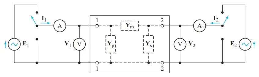
Figure 1 Determining the short-circuit admittance parameters
To prevent source E2 from affecting the measurement of the input admittance, we set the right-hand switch in Figure 1 so that the ammeter measuring I2 shorts the output terminals (port 2). Similarly, when we apply E2 to the output terminals, we set the left-hand switch to connect the ammeter measuring I1 directly across the input terminals (port 1), thus shorting them.
With E1 applied to the input terminals, we can use the readings of the meters in the input circuit to find an I/V ratio that represents the input admittance of the network with the output terminals short-circuited. The reading on the ammeter measuring I2 indicates that a portion of the input current is coupled through to the output.
Looking back into the short-circuited output terminals, we see a Norton-equivalent source containing a dependent current source controlled by the voltage applied to the input terminals. To find the parameter that relates I2 to E1, we simply divide I2 by V1, giving a quantity in Siemens.
By reversing the position of the switches, we can find similar parameters for the output terminals. Thus, there are four short-circuit admittance parameters for any four-terminal, two-port network:
Short-circuit input admittance:
\[\begin{matrix}{{\text{y}}_{\text{11}}}\text{=}\frac{{{\text{I}}_{\text{1}}}}{{{\text{E}}_{\text{1}}}}\left( with\text{ }{{\text{E}}_{\text{2}}}=0 \right) & {} & \left( 1 \right) \\\end{matrix}\]
Short-circuit reverse-transfer admittance:
\[\begin{matrix}{{\text{y}}_{\text{12}}}\text{=}\frac{{{\text{I}}_{\text{1}}}}{{{\text{E}}_{\text{2}}}}\left( with\text{ }{{\text{E}}_{\text{1}}}=0 \right) & {} & \left( 2 \right) \\\end{matrix}\]
Short-circuit forward-transfer admittance:
\[\begin{matrix}{{\text{y}}_{21}}\text{=}\frac{{{\text{I}}_{\text{2}}}}{{{\text{E}}_{\text{1}}}}\left( with\text{ }{{\text{E}}_{\text{2}}}=0 \right) & {} & \left( 3 \right) \\\end{matrix}\]
Short-circuit forward-transfer admittance:
\[\begin{matrix}{{\text{y}}_{\text{22}}}\text{=}\frac{{{\text{I}}_{\text{2}}}}{{{\text{E}}_{\text{2}}}}\left( with\text{ }{{\text{E}}_{\text{1}}}=0 \right) & {} & \left( 4 \right) \\\end{matrix}\]
Since a Norton-equivalent current source has to be in parallel with the input admittance, the equivalent circuit has two paths for I1 to follow between the input terminals. Writing the Kirchhoff’s current-law equation for I1 gives
$\begin{matrix}{{\text{y}}_{\text{11}}}{{\text{E}}_{\text{1}}}\text{+}{{\text{y}}_{\text{12}}}{{\text{E}}_{\text{2}}}\text{=}{{\text{I}}_{\text{1}}} & {} & \left( 5 \right) \\\end{matrix}$
Similarly, for the output terminals (port 2),
\[\begin{matrix}{{\text{y}}_{\text{21}}}{{\text{E}}_{\text{1}}}\text{+}{{\text{y}}_{\text{22}}}{{\text{E}}_{\text{2}}}\text{=}{{\text{I}}_{2}} & {} & \left( 6 \right) \\\end{matrix}\]
Figure 2 shows the y-parameter equivalent circuit that satisfies Equations 5 and 6.
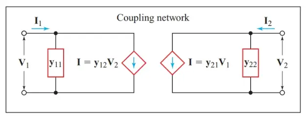
Figure 2 y-parameter equivalent circuit
We can now find the y-parameters for the p-network shown with dashed lines in Figure 1. When the ammeter measuring I2 shorts the output terminals,
${{\text{I}}_{\text{1}}}\text{=}{{\text{E}}_{\text{1}}}\left( {{\text{Y}}_{\text{p}}}\text{+}{{\text{Y}}_{\text{m}}} \right)$
And
\[\begin{matrix}{{\text{Y}}_{\text{p}}}\text{+}{{\text{Y}}_{\text{m}}}\text{=}\frac{{{\text{I}}_{\text{1}}}}{{{\text{E}}_{\text{1}}}}\text{=}{{\text{y}}_{\text{11}}} & {} & \left( 7 \right) \\\end{matrix}\]
Similarly,
\[\begin{matrix}{{\text{Y}}_{\text{s}}}\text{+}{{\text{Y}}_{\text{m}}}\text{=}\frac{{{\text{I}}_{\text{2}}}}{{{\text{E}}_{\text{2}}}}\text{=}{{\text{y}}_{22}} & {} & \left( 8 \right) \\\end{matrix}\]
When the meter measuring I1 is connected directly across the input terminals, there can be no voltage drop across Yp and, hence, no current through Yp. Therefore, all the current through Ym must flow through the ammeter in the input circuit. As a result, I1 has the same magnitude as the current through Ym. But the current through Ym is caused by E2 and has the opposite direction to I1, as shown in Figure 1. Hence,
${{\text{I}}_{\text{1}}}\text{=-}{{\text{Y}}_{\text{m}}}{{\text{E}}_{\text{2}}}$
And
\[\begin{matrix}{{\text{Y}}_{\text{m}}}\text{=-}\frac{{{\text{I}}_{\text{1}}}}{{{\text{E}}_{\text{2}}}}\text{=-}{{\text{y}}_{\text{12}}} & {} & \left( 9 \right) \\\end{matrix}\]
Similarly,
\[\begin{matrix}{{\text{Y}}_{\text{m}}}\text{=-}\frac{{{\text{I}}_{\text{2}}}}{{{\text{E}}_{\text{1}}}}\text{=-}{{\text{y}}_{\text{21}}} & {} & \left( 10 \right) \\\end{matrix}\]
Rearranging Equations 7 to 10 gives the equivalent π-network in terms of the y-parameters of the coupling network:
\[\begin{align}& \begin{matrix}{{Y}_{m}}=-{{y}_{12}}=-{{y}_{21}} & {} & \left( 11 \right) \\\end{matrix} \\& \begin{matrix}{{Y}_{p}}={{y}_{11}}+{{y}_{12}} & {} & \left( 12 \right) \\\end{matrix} \\& \begin{matrix}{{Y}_{s}}={{y}_{22}}+{{y}_{21}} & {} & \left( 13 \right) \\\end{matrix} \\\end{align}\]
Summary
The short-circuit admittance parameters of a two-port network can be determined by representing the network by its equivalent π-network.