What is a Nyquist Stability Criterion?
The Nyquist stability criterion is a frequency domain tool that is used in the study of stability. To use this criterion, the frequency response data of a system must be presented as a polar plot in which the magnitude and the phase angle are expressed as a function of frequency.
Nyquist Theorem
In 1932, H. Nyquist used a theorem by Cauchy regarding the function of complex variables to develop a criterion for the stability of the control system. Cauchy’s theorem is concerned with mapping contours from one complex plane to another. Since we are interested in the presence of roots of the characteristic equation in the right half of the s-plane, we will be mapping contours that enclose the right half-plane. The characteristics equation
$1+GH(s)=0$
Is a function F(s) of the complex variable s set equal to zero, that is
$F(s)=1+GH(s)=0$
The above equation can also be expressed as
\[F(s)=\frac{K(s+{{z}_{1}})(s+{{z}_{2}})\cdots (s+{{z}_{n}})}{(s+{{p}_{1}})(s+{{p}_{2}})\cdots (s+{{p}_{m}})}=0\]
Where the -zi’s are the roots of the characteristics equation and the –pi’s are the poles of the corresponding open loop transfer function GH(s). We first map the contours of the s-plane into the (1+GH)-plane, then for convenience, we omit the 1 of (1+GH) and map the contours into the GH-plane. The resulting contours provide information on the existence of roots that have a positive real part, that is, that are located in the right-half plane.
- You May Also Read: Root Locus Method | Root Locus Matlab
Cauchy’s Theorem
A theorem by Cauchy can provide information about the number of zeros of a function F(s) having positive real parts. In our study of stability, we will be applying the theorem to the characteristic equation of the system expressed as
$F(s)=1+GH(s)=0\text{ (1)}$
Where F(s) is often given as
\[F(s)=\frac{K(s+{{z}_{1}})(s+{{z}_{2}})\cdots (s+{{z}_{n}})}{(s+{{p}_{1}})(s+{{p}_{2}})\cdots (s+{{p}_{m}})}=0\text{ (2)}\]
As applied to equation (1) and (2), Cauchy’s theorem is as follows:
If :
- We map a contour in the s-plane that encircles z zeros and p poles of F(s),
- The contour does not pass through any poles or zeros of F(s), and
- The transversal along the contour in the s-plane is clockwise,
Then,
The corresponding contour (or image) in the F(s)-plane encircles the origin N=Z-P times in the clockwise direction.
The theorem is summarized by
N= Z-P (3)
Where
P= the number of poles of F(s)
Z=the number of zero (roots) of F(s)
N = the number of clockwise encirclements of the origin in the F(s)-plane.
It is convenient to map with GH(s) rather than 1+ GH(s) =F(s). For the GH(s) mapping, equation (3) applies, if we let N=the number of clockwise encirclements of the -1 point in the GH-plane. For the majority of the applications, we know GH(s) in the factored form:
$GH(s)=\frac{K(s+{{s}_{1}})(s+{{s}_{2}})\cdots }{(s+{{p}_{1}})(s+{{p}_{2}})\cdots }$
Where –si’s are the zeros of the open-loop transfer function. By finding the image in the GH-plane rather than the F(s) plane, we avoid adding 1 to each of the computation.
The stability of a control system is determined by searching the right-half of the s-plane for zero (roots) of the characteristics equation:
$F(s)=1+GH(s)=0$
If there are no roots in the right half plane, then the system is stable.
Now we shall establish the procedure for searching the right-half plane and relating the stability of the control system to the polar plot. The positive jω-axis in the s-plane, used for the polar plot, will be expanded to a contour enclosing the entire right half-plane.
The contour, shown in the following figure, consists of three parts.
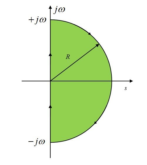
Figure1. Nyquist Contour
- The positive jw-axis
- The negative jw-axis
- A semi-circle of infinite radius R
Nyquist Contour
The complete contour, enclosing the entire right half-plane, is called the Nyquist contour.
A smaller radius could be used if we knew that there were no roots of the characteristics equation beyond the semi-circle.
We use GH(s)-plane, which is
$F(s)-1=GH(s)$
To map the Nyquist contour of the s-plane into the GH-plane. This change in the mapping function is convenient because we usually know GH(s) in the factored form as,
$GH(s)=\frac{K(s+{{s}_{1}})(s+{{s}_{2}})\cdots }{(s+{{p}_{1}})(s+{{p}_{2}})\cdots }$
Nyquist Stability Criterion
The Nyquist stability criterion can now be stated:
When the Nyquist contour is mapped into the GH-plane by the open-loop transfer function GH(s) of a system, then one of the following two cases applies:
Case 1:
When no poles of GH(s) are in the right half of the s-plane, the corresponding feedback control system is stable if and only if the control of the image of the Nyquist contour does not circle the (-1+j0) point in the GH-plane.
Case 2:
When the number of poles of GH(s) in the right half of the s-plane is not zero, the corresponding feedback control system is stable if and only if the contour of the image of the Nyquist contour encircles the (-1+j0) point in a counter-clockwise direction by an amount equal to the number of poles of GH(s) with positive real parts.
The basis of these two cases is:
N=Z-P
For case 1, where P=0 we have N=Z, that is, the number of zeros is equal to the number of encirclements. For a stable system, N must be zero.
For case 2, N=Z-P results in N=-P, since Z=0 for a stable system.
What is a Nyquist Plot?
A Nyquist plot, known as a polar plot, is a frequency response of a linear system, which means we replace s with jω in a transfer function G(s).
In order to draw a polar plot for transfer function G (jω) for the frequency range 0 to infinity, we need to be recognizant of the following four important points;
- Start of plot where ω=0
- End of plot where ω=∞
- Where the plot crosses the real axis, i.e.,
Imaginary (G(jω))=0
- Where the plot crosses the imaging axis, i.e.,
Real (G(jω))=0
Nyquist Stability Criterion Example
Consider the first-order control system
\[G(s)=\frac{1}{1+sT}\]
Where T is the time constant.
Let’s represent function G(s) in terms of frequency response G (jω) by substituting s = jω:
$G(j\omega )=\frac{1}{1+j\omega T}$
The magnitude |G (jω)| is obtained as:
$\left| G(j\omega ) \right|=\frac{1}{\sqrt{1+{{\omega }^{2}}{{T}^{2}}}}$
The phase of G (jω), expressed by φ, is calculated as:
$\angle G(j\omega )=-arctan(\omega T)$
Start of plot where ω=0
$\left| G(j\omega ) \right|=\frac{1}{\sqrt{1+0}}=1$
$\phi ={{\tan }^{-1}}\left( \frac{0}{1} \right)=0$
End of plot where ω=∞
$\left| G(j\omega ) \right|=\frac{1}{\sqrt{1+\infty }}=0$
$\phi ={{\tan }^{-1}}\left( \frac{-\infty }{1} \right)=-{{90}^{\centerdot }}$
The mid part of the plot where ω = 1/T
$\left| G(j\omega ) \right|=\frac{1}{\sqrt{1+1}}=\frac{1}{\sqrt{2}}$
$\phi ={{\tan }^{-1}}\left( \frac{-1}{1} \right)=-{{45}^{\centerdot }}$
Let’s combine the above points in a table,
| Value of ω | $\left| G(j\omega ) \right|$ | $\angle G(j\omega )$ |
| ω=0 | 1 | 0 |
| ω = 1/T | $\frac{1}{\sqrt{2}}$ | $-{{45}^{\centerdot }}$ |
| ω=∞ | 0 | $-{{90}^{\centerdot }}$ |
So, for the first-order system, the polar plot will look like:
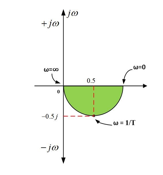
Figure 2. Polar Plot for First-Order System