Learn about the transient response of first and second order systems and how the time constant influences their response characteristics.
In control systems, a transient response (which is also known as a natural response) is the system response to any variation from a steady state or an equilibrium position. The examples of transient responses are step and impulse responses which occur due to a step and an impulse input respectively.
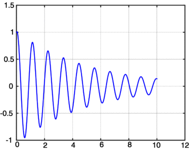
Damping Oscillation: A typical Transient Response Example
For a system with transfer function G(s), whether open loop or closed loop and input R(s), the output is
\[C\left( s \right)=\text{ }G\text{ }\left( s \right)\text{ }R\left( s \right)\]
For distinct poles, whether real or complex, the partial fraction expansion of C(s) and the corresponding solution c(t) are, from
\[C\left( s \right)=\frac{{{K}_{1}}}{\left( s+{{p}_{1}} \right)}+\frac{{{K}_{2}}}{\left( s+{{p}_{2}} \right)}+\ldots +\frac{{{K}_{n}}}{\left( s+{{p}_{n}} \right)}\text{ (1)}\]
$c\left( t \right)={{K}_{1}}\exp \left( -{{p}_{1}}t \right)+{{K}_{2}}\exp \left( -{{p}_{2}}t \right)+\ldots +{{K}_{n}}\exp \left( -{{p}_{n}}t \right)$
The denominator of C(s)= G(s)R(s) and its partial faction expansion contain terms due to the poles of input R(s) and those of the system G(s). The terms due to R(s) yield the forced solution whereas the system poles give the transient solution, and this is the part of the response into which more insight is needed.
System Stability
This is the most important characteristic of the transient response. For a system to be useful, the transient solution must decay to zero. This leads to the following definition,
A system is stable if transient solution decays to zero and is unstable if this solution grows.
The fundamental stability theorem can be formulated by examination of (1). If any system pole –pi is positive or has a positive real part, then the corresponding exponential grows, so the system is unstable. A positive real part means that the pole lies in the right half of the s-plane. Hence;
A system is stable if and only if all the system poles lie in the left half of the s plane.
Transient Response First Order System (Simple Lag)
The first order system shown in the following figure is very common for analysis purposes in control system.
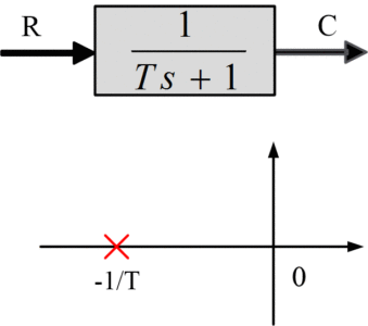
Figure 1: First Order System
For a step input R(s) =1/s,
\[C(s)=\frac{{}^{1}/{}_{T}}{s(1+{}^{1}/{}_{T})}=\frac{{{K}_{1}}}{s}+\frac{{{K}_{2}}}{s+{}^{1}/{}_{T}}\]
${{K}_{1}}={{\left. \frac{{}^{1}/{}_{T}}{s+{}^{1}/{}_{T}} \right|}_{s=0}}=1$
${{K}_{2}}={{\left. \frac{{}^{1}/{}_{T}}{s} \right|}_{s=-{}^{1}/{}_{T}}}=-1$
Hence the transient response would be,
\[c\left( t \right)=1-{{e}^{-{}^{t}/{}_{T}}}\]
In the above transient response, first term indicates the forced solution because of the input while the second term indicates the transient solution, because of the system pole. Figure 2 demonstrates this transient (second term) and c(t). It can be clearly seen in figure 2 (a) that the transient is a decaying exponential; if the response takes long to decay, then the system’s overall response is slow, hence we can say that the response decay speed is of significant importance. The speed of decay is usualy measured in terms of time constant.
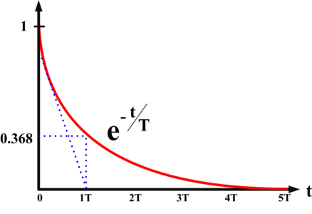
Fig. 2(a): Step Response of Simple Lag Network
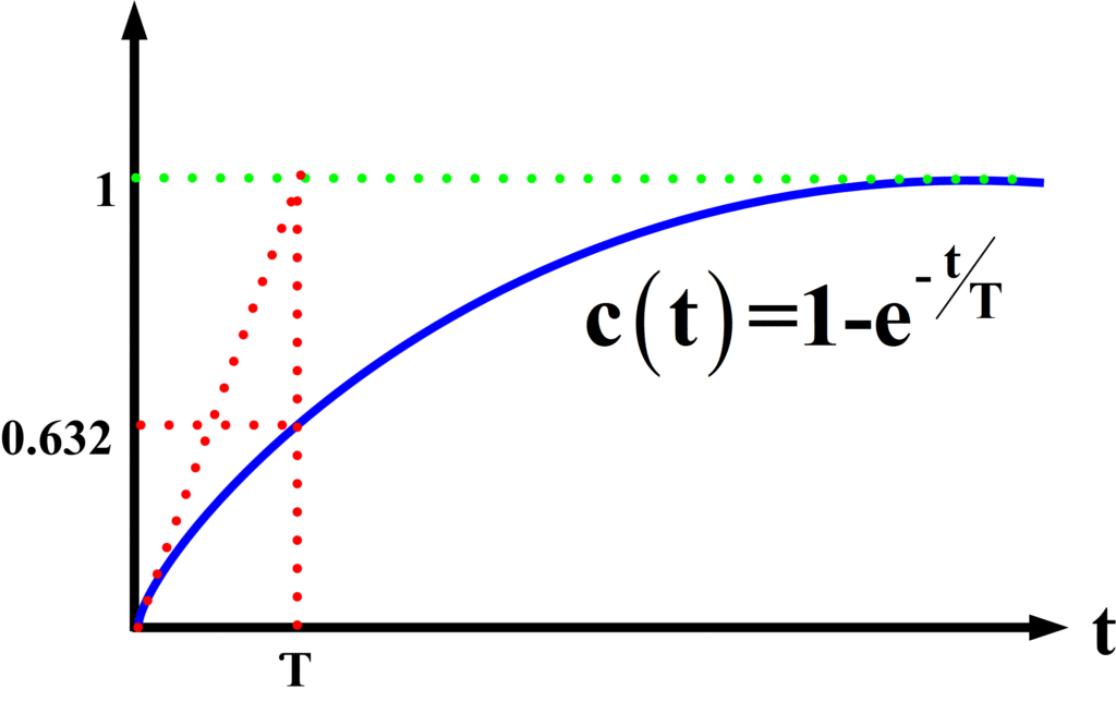
Fig. 2(b): Step Response of Simple Lag Network
Time Constant of Second Order System
The time it takes, in seconds, for the decaying exponential to be decreased to e-1 =0.368 of its initial value.
Because e-t/T= e-1 when t=T, it can be observed that:
- The time constant of a simple lag network (1/Ts+1) is T seconds.
- This is the reason that a general lag transfer function is written in this particular form. The coefficient of s shows the speed of decay of a response.
- Usually, in 4T seconds, the transient response decays to 1.8% of its initial value.
- At t= T,
c (T)=1-0.368=0.632
The values at t=T provide one point for sketching the curves in figures (2a,2b). Also the curves are initially tangent to the dashed lines, since
\[\frac{d}{dt}\left( {{e}^{-{}^{t}/{}_{\tau }}} \right){{|}_{t=0}}=-\frac{1}{T}{{e}^{-{}^{t}/{}_{T}}}{{|}_{t=0}}=-\frac{1}{T}\]
These two facts provide a good sketch for the response.
Now consider the correlation between this response and the pole position at s=-1/T in Fig .1. The purpose of developing such insight is that it will permit the nature of the transient response of a system to be judged by inspection of the pole-zero pattern.
For the simple-lag network, two characteristics are crucial:
Stability
As discussed, for stability, the system pole -1/T must lie the left half of the s-plane, since otherwise the transient e-t/T grows instead of decays as t increases.
Speed Of Response
In order to speed up the system response (that is by reducing its time constant T), the pole -1/T must be moved on the left side of the s-plane.
Transient Response of Second Order System (Quadratic Lag)
This very common transfer function to represent the second order system can be reduced to the standard form
\[G\left( s \right)=\frac{\omega _{n}^{2}}{{{s}^{2}}+2\zeta {{\omega }_{n}}s+\omega _{n}^{2}}\]
Where
ωn = undraped natural frequency
ζ = damping ratio
For a unit step input which is R(s) =1/s, the transform of the output would be
\[C\left( s \right)=\frac{\omega _{n}^{2}}{s({{s}^{2}}+2\zeta {{\omega }_{n}}s+\omega _{n}^{2})}\]
The characteristic equation would be
${{s}^{2}}+2\zeta {{\omega }_{n}}s+\omega _{n}^{2}=0$
These system poles depend on ζ:
$\zeta >1:overdamped:{{s}_{1,2}}=-\zeta {{\omega }_{n}}\pm {{\omega }_{n}}\sqrt{{{\zeta }^{2}}-1}$
$\zeta =1:critically~damped:{{s}_{1,2}}=-{{\omega }_{n}}$
$\zeta <1:underdamped:{{s}_{1,2}}=-\zeta {{\omega }_{n}}\pm j{{\omega }_{n}}\sqrt{1-{{\zeta }^{2}}}$
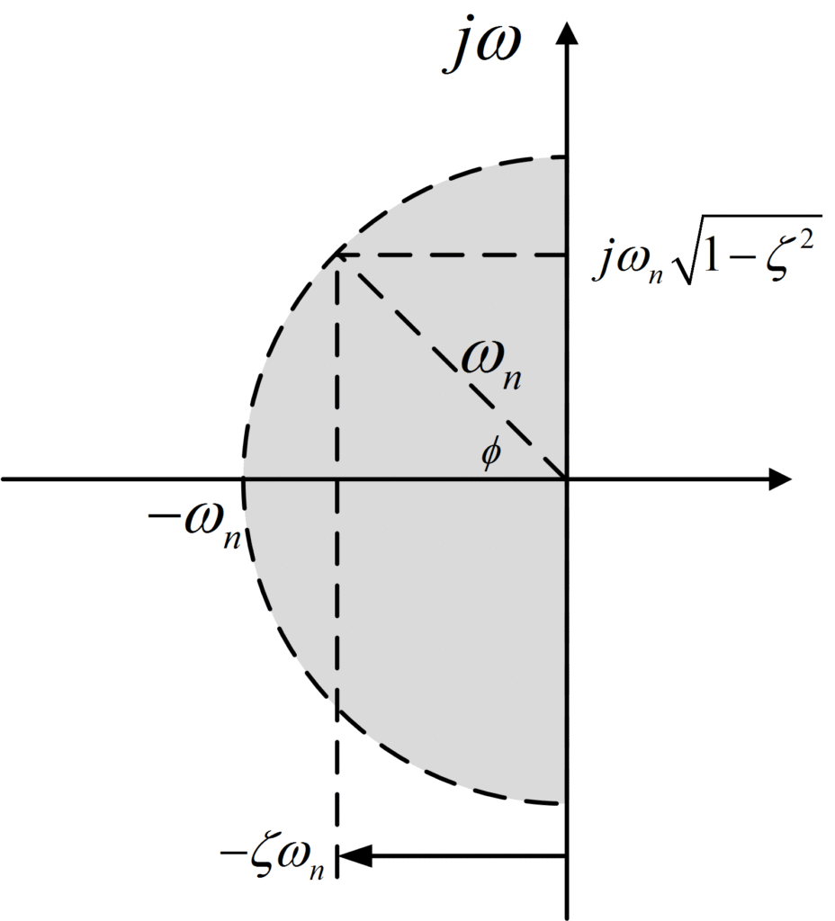
Figure 3: System Poles Quadratic Lag
Figure 3 shows the s-plane for plotting the pole positions.
- For ζ>1, these are on the negative real-axis, on both sides of -ωn .
- For ζ=1, both poles coincide at -ωn.
- For ζ<1, the poles move along a circle of radius ωn centered at the origin, as may be seen from the following expression for the distance of the poles to the origin:
$\left| {{s}_{1,2}} \right|={{\left[ {{\left( \zeta {{\omega }_{n}} \right)}^{2}}+{{\left( {{\omega }_{n}}\sqrt{1-{{\zeta }^{2}}} \right)}^{2}} \right]}^{{}^{1}/{}_{2}}}={{\omega }_{n}}$
From the geometry in figure 3, it is seen also that
$Cos\left( \theta \right)=\frac{\zeta {{\omega }_{n}}}{{{\omega }_{n}}}=\zeta $ Hence,
The damping ratio $\zeta =\cos \phi $ , where ∅ is the position angle of the poles with the negative real axis.
Time Constant
This is the time constant in seconds for the amplitude of oscillation to decay to e-1 of its initial value:${{e}^{-\zeta {{\omega }_{n}}t}}={{e}^{-1}}$, Hence
\[T=\frac{1}{\zeta {{\omega }_{n}}}\]
Analogous to the simple lag, the amplitude decays to 2% of its initial value in 4T seconds. It is again important to determine the correlation between dynamic behavior and the pole positions in the s-plane in Figure 3:
Absolute Stability
The real part $-\zeta {{\omega }_{n}}$ of the poles must be negative for the transient to decay; that is, the poles must lie in the left half of the s-plane.
Relative Stability
To avoid excessive overshoot and unduly oscillatory behavior, damping ratio ζ must be adequate. Since ζ = Cosϕ, the angle ϕ may not be close is 90o.
Time Constant Effect
The time constant is reduced (that is, the speed of decay of the transient is increased) by increasing by increasing the negative real part of the pole position.
Speed of Response
The speed of response of the system is increased by increasing the distance ωn of the poles to the origin.
Undamped Natural Frequency
This equals the distance of the poles to the origin. Moving the poles out radially (with ζ constant) increases the speed of response while the percentage overshoot remains constant.
Frequency of Transient Oscillations ${{\omega }_{n}}\sqrt{1-{{\zeta }^{2}}}$
This frequency also called the resonance frequency or damped natural frequency equals the imaginary part of the pole positions.
Key Takeaways
First and second-order systems demonstrate different transient responses based on their time constants. The time constant determines the rate at which the system responds to input changes, influencing factors like settling time, rise time, and overshoot in the system’s response.