When operated as a generator, the armature of the DC machine is driven by a prime mover. As the armature coils move through the flux created by the stator field, a voltage is induced in them. To understand the operation of the DC generator we need a specific relationship for the generated voltage in terms of the flux, the physical design of the machine, and its speed.
Generated voltage
Faraday’s law tells us
\[\begin{matrix} {{E}_{a}}=N\frac{d{{\phi }_{p}}}{dt}\text{ }or\text{ }{{E}_{a}}=N\frac{\Delta {{\phi }_{p}}}{\Delta t} & {} & \left( 1 \right) \\\end{matrix}\]
Where N is the number of series conductors.
Rather than use the derivative form of equation 1, we can use the different form. During each revolution, a conductor cuts the flux of P poles, where P is the number of poles in the machine. Thus, the total amount of flux cut in one revolution is
\[\begin{matrix} \Delta \phi =P{{\phi }_{p}} & {} & \left( 2 \right) \\\end{matrix}\]
Where ϕp is the flux per pole.
If the speed of the machine in RPM is represented by n, then the time to complete one revolution is
\[\begin{matrix} \Delta t=\frac{1}{{}^{n}/{}_{60}}=\frac{60}{n} & {} & \left( 3 \right) \\\end{matrix}\]
Substituting equations 2 and 3 into 1 yields
\[\begin{matrix} {{E}_{a}}=NP{{\phi }_{p}}\frac{n}{60} & {} & \left( 4 \right) \\\end{matrix}\]
To find the number of series conductors in the armature winding, let Za be the total number of armature conductors and a be the number of parallel paths.
We have seen that the number of parallel paths in the armature winding is equal to the number of poles for a lap winding and is 2 for a wave winding.
The number of series conductors is
\[\begin{matrix} N=\frac{{{Z}_{a}}}{a} & {} & \left( 5 \right) \\\end{matrix}\]
Equation 5 can be substituted into equation 4 to yield an expression for the generated voltage of a DC generator:
\[\begin{matrix} {{E}_{a}}=\left( \frac{P{{Z}_{a}}}{60a} \right)n{{\phi }_{p}}={{K}_{g}}n{{\phi }_{p}} & {} & \left( 6 \right) \\\end{matrix}\]
Where
\[\begin{matrix} {{K}_{g}}=\frac{P{{Z}_{a}}}{60a} & {} & \left( 7 \right) \\\end{matrix}\]
Equation 6 is called the generated voltage equation for a DC generator and is an extremely important equation for the DC generator.
Kg is called the generator constant for a DC machine and is solely a function of the design of the machine— specifically, the number of poles and the type of winding. We can note several things about the voltage equation:
-
Because of saturation effects in the iron of the machine, the flux per pole is a nonlinear function of the field current.
-
Ea is a linear function of the flux per pole, so it is also nonlinear with respect to the field current.
-
Ea is linear with respect to the rotational speed of the machine—to in radians/s or n in RPM.
DC Generator Characteristics Curves
Figure 1 shows relationships between generated voltage, field current, ϕ, and speed. The relationship between the flux per pole and the field current is shown in Figure 1 (a). Because the stator structure is ferromagnetic, it will exhibit the effects of both hysteresis and saturation. Thus, the flux shows both of these effects.
As the field current is increased, the flux increases until saturation of the core cause the flux to roll off. When the field current is then decreased, the domains within the steel are already aligned, so there is more flux when the field current is decreased than when it is increased.
Because the voltage is directly proportional to the flux, as shown by equation 5, the voltage will also exhibit hysteresis and saturation as the field current is changed with the machine running at constant speed. The magnetization curve is described in more detail in the next section.
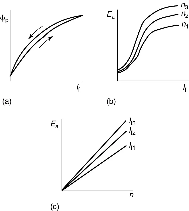
FIGURE 1: DC Generator Characteristics Curves
Figure 1(b) shows the voltage as a function of field current; however, the hysteresis effect has been omitted. Three voltage curves are shown for three machine operating speeds, n 1 < n 2 < n3. Finally, Figure 1(c) shows the voltage as a function of speed for three values of field current.
The relationship between generated voltage and speed is linear if the field current (and thus the flux) is held constant. Because the generated voltage is directly proportionate to the speed of the machine, the voltage-speed curve passes through the origin.
DC Generator Magnetization Curve
Figure 2 showed the equivalent circuit for a separately excited DC generator. The field is supplied from a separate DC source that is applied to the shunt field of the machine.

FIGURE 2: Complete equivalent circuit of a separately excited DC generator.
The variation of the generated voltage, Ea, with the field current is shown by the magnetization curve or open-circuit characteristic, as shown in Figure 1(b).
The magnetization curve is obtained by driving the machine at a constant speed and varying the field current.
Assuming the field has been previously energized, the steel of the stator pole-faces will have some residual magnetism. This provides some flux, so the machine will have an output of a few volts even with the field circuit disconnected.
As the field current is increased, the flux is almost directly proportionate to the field current, so the voltage increases linearly with the field current. As the steel in the machine begins to saturate, however, the curve will bend over.
After some maximum value of field current is reached, reducing the field current will cause hysteresis to be observed—the voltage output of the machine will be higher when the current is decreased than it was when the current was increased. This difference may be only a few volts but is an easily observed demonstration of hysteresis.
The magnetization curve only has to be done at one speed because we can obtain one at any other speed from the equation for the generated voltage. Consider if we have two voltages at two different speeds, with the flux per pole held constant:
$\begin{matrix} {{E}_{a1}}={{K}_{g}}{{\phi }_{p}}{{n}_{1}} & {} & \left( 8 \right) \\\end{matrix}$
$\begin{matrix} {{E}_{a2}}={{K}_{g}}{{\phi }_{p}}{{n}_{2}} & {} & \left( 9 \right) \\\end{matrix}$
Dividing (8) by (9) and rearranging yields
\[\begin{matrix} {{E}_{a2}}={{E}_{a1}}\frac{{{n}_{2}}}{{{n}_{1}}} & {} & \left( 10 \right) \\\end{matrix}\]
Equation 10 allows us to easily calculate the generated voltage at any speed if we know it for one speed, assuming the field current is held constant.
Voltage Regulation
The terminal voltage for the separately excited DC generator shown in Figure 2 can be found by writing a voltage loop equation:
$\begin{matrix} {{V}_{t}}={{E}_{a}}-{{I}_{a}}{{R}_{a}} & {} & \left( 11 \right) \\\end{matrix}$
If the field voltage is kept constant, the field current and the flux per pole, ϕp, will also be constant.
If the generator is driven at constant speed, the internal voltage, Ea, will be constant, since all the terms on the right-hand side of equation 6 are constant. Under these conditions, equation 11 represents a linear relationship between the terminal voltage and the armature current, with a negative slope. Thus, as the armature load current increases, the terminal voltage will decrease linearly, as shown by the solid line in Figure 3.

FIGURE 3: Variation of terminal voltage with load current for a separately excited DC generator.
Generators are designed to produce rated voltage when delivering rated load current. For the separately excited generator, the terminal voltage is above the rated voltage at less than full load. To quantify the variation of terminal voltage with output, we define the voltage regulation, VR, in the same manner as for the transformer:
\[\begin{matrix} VR=\frac{{{V}_{nl}}-{{V}_{fl}}}{{{V}_{fl}}}\times 100 & {} & \left( 12 \right) \\\end{matrix}\]