This section briefly describes matters concerned with transmission lines in electrical networks. Knowledge of the material described here is very useful for the technical personnel in electricity and its generation and distribution.
Inductive and Capacitive Effect
In addition to the ohmic resistance in the wires and electric conductors, conductors carrying AC electricity have inductive and capacitive effects.
Consider, for instance, a pair of transmission lines that extend for several miles and compare them to two plates forming a capacitor. You will see that there is a similarity in terms of the two metallic surfaces, being at a distance from each other, with a common cross-section area separated by a nonconductive material (air). Thus, the two conductors form a capacitor.
The same thing is true for the magnetic effect of the current in each conductor on itself and on the other conductor. Thus, there exists an inductance between the two conductors.
The amount of capacitive and inductive effects might be small and negligible for short wires, for example, in the household wiring having a low voltage, but they are not negligible for the very long transmission lines and the high voltages they carry.
Capacitive and inductive effects of the transmission lines, thus, need to be included in the calculation of their current and voltage drop. If these effects are added, the schematic representation of an electric network between load(s) and the source(s) is similar to Figure 1b, instead of Figure 1a.
Resistances and inductances are in series with each other along the length of a conductor, but the capacitive effects are shown as parallel. These effects are indicated for one line only, but they correspond to both conductors.
In practice, there are usually more than two conductors, particularly for three-phase lines. But, for three-phase systems, the effects of two conductors do not add up as in the case of single-phase wires because there are no return lines carrying the exact same currents at the same moment.
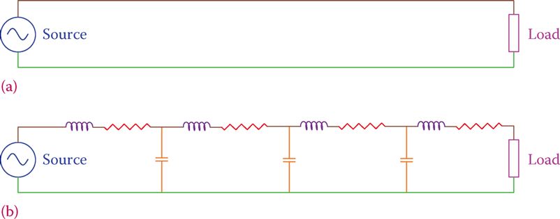
Figure 1 Typical representation of a transmission line. (a) Two long transmission wires for AC. (b) Assumed capacitors and inductors to represent the capacitance and inductance effects of the nearby wires in AC transmission.
Values for ohmic resistance can be readily defined for each conductor in terms of its length, cross-section area, the conductor material, and its specific resistance. These data are usually available for any cable in terms of the resistance for each meter of the conductor, or 1000 ft of it.
Capacitor value and inductor value for a set of conductors, however, depending on the factors particular to their setup. Depending on conductors spacing, their radii, the way they are laid out, the number of conductors, and how many are in each bundle sharing the same current, a value can be determined for the inductance of a given length (e.g., 1 km or 1 mile) of a transmission line.
Similarly, a value can be obtained for the capacitance. In this way, more precise values for the current, voltage drop, lost energy, and so on can be found for a transmission line of a given length.
Corona Effect
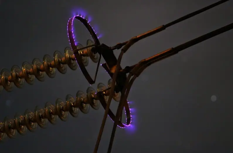
Another phenomenon that causes a loss in transmission lines is corona. Corona is the effect of potential difference (voltage) on the air surrounding the transmission lines, ionizing the air. This effect reflects in the form of a glow coming out of lines.
Corona depends on the voltage and spacing between the wires. The amount of energy lost this way, however, is small and is often neglected.
Corona: Corona is a local electric discharge around the conductors of high-voltage transmission lines when the (especially humid) air is ionized. It is manifested by a bluish glow and a small humming sound. This phenomenon is accompanied by a slight loss of power used for making the sound and the glow.
Figure 2 illustrates the relative spacing of possible transmission lines arrangements. Figure 2a shows a general case where the three lines of a three-phase system are at locations 1, 2, and 3. These lines, furthermore, are at general distances D12, D13, and D23 from each other.
In the discussions that follow it is assumed that the loads on the three phases are the same and we are dealing with balanced loads. Except in the case of Figure 2c where all lines are equidistance from each other, values for the inductance and capacitance of a length of the lines are not the same. As a result, voltage drops in the three lines are different. Consequently, at the load site, the voltage at the three lines carrying three phases are not the same. Also, the phase relationships can be disturbed and the three phases will no longer be 120° from each other.
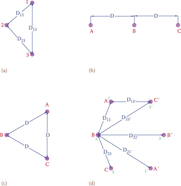
Figure 2 Conductor positions in some common three-phase transmission lines. (a) In three corners of a triangle. (b) Along one horizontal line. (c) At the three corners of an equilateral triangle. (d) Double-circuit three-phase, as on transmission structures.
It is very undesirable if the voltages arriving at a site from the same source are different and a proper three-phase system is not delivered at the line end.
Transposition Effect
In many arrangements for transmission lines, it is not common, and sometimes impossible, to have the lines at the corners of an equilateral triangle (e.g., Figure 2b and d). To overcome this problem, it is common practice to rotate the lines, so that each of the phases occupies the same physical position equally along the length of the transmission line. In this way, the total inductance and capacitance of all three lines will be equalized. This rotation is called transposition, and a line treated this way is said to be transposed. This is illustrated in Figure 3, which illustrates that each of the three-phase lines A, B, and C are placed equally in the three physical positions denoted by 1, 2, and 3 along the length of the transmission line.
When all the three phases of a line equally occupy the three positions, so that all the voltage differences cancel each other, the line is said to be completely transposed.
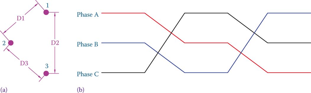
Figure 3 Transposition in transmission lines. (a) The physical position of the three-phase lines. (b) Interchanging the wire positions at some point along the line.
Transposition: a Special arrangement in the transmission of three-phase power, in which the wires are rotated such that the location of wires for each phase is physically interchanged so that each wire equally occupies the same location as the other wires within the length of a line.
In all that follows we assume that the lines are solid, circular, and all have the same radius r. The distances are denoted by D with one or two indexes when necessary (like in D12).
The numbers calculated for inductance and capacitance are for a given length, and, thus, for the whole length of a transmission line, they must be multiplied by the line length. Results of the calculations are per phase for three-phase lines.
In single-phase systems, the numbers must be doubled for inductance and halved for capacitance because there are two lines and one is the return of the other line.
Before going ahead, we need to define the two following terms. In fact, these are the parameters that change, from the one-line arrangement to another.
Geometrical mean distance (GMD) is a number corresponding to the equivalent distance between two or more lines (cables). Geometrical mean radius (GMR) is a number corresponding to the effective radius of one or more lines.
Geometrical mean distance (GMD): A term in power transmission lines corresponding to the spacing between the two (in a single phase) and three or six (in three phase) power lines used to determine the inductance and capacitance associated with lines.
Geometrical mean radius (GMR): Term in power transmission lines corresponding to the size (radius) of power lines used to determine their associated inductance and capacitance.
Line Inductance
The following general formula can be used for finding the inductance of each line in a transmission system. If three phases, the line is assumed to be transposed and the load(s) balanced.
$\begin{matrix}L=\left( 2\times {{10}^{-7}} \right)\ln \left( \frac{GMD}{GMR} \right) & {} & \left( 1 \right) \\\end{matrix}$
GMD and GMR are as defined above, and they vary on a case-by-case basis. The coefficient (2 × 10⁻⁷) is for the metric system, and the answer is in henries per meter. For the imperial system, a conversion is necessary, as will be seen later in some examples. We consider GMD and GMR for the following three cases:
The logarithm of a Number
Using logarithms is a useful tool in many engineering and other subjects. It makes calculations and solution to problems easier. Here we briefly explain what a logarithm is and show some examples.
There are two logarithms, and we may say any positive number has two logarithm values. The difference between them is the base number, and it is possible to change from one logarithm to the other.
The two logarithms are decimal logarithm, which has a base 10, and the natural logarithm whose base is another number. We first start with the decimal logarithm, and when you understand it well, it is easy to understand the other. Indeed, the logarithm is the opposite of exponential power.
Decimal Logarithm
To show the decimal logarithm of a number, the symbol “log” is used, such as log 10, log 20, etc. Consider the following relationships. You may want to check them on a calculator:
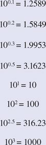
In conjunction with the above relationships and in the same order you can write
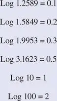
From the above examples, it is clear that if y = 10x, then x = log y.
Now that the notion of logarithm function is clear for you, try some negative numbers for the x and see the result on y. All values found this way is smaller than 1.0. Also, remember that negative numbers do not have logarithm. You will get an error message if try to find the log of a negative number on the calculator.
Now, we consider GMD and GMR for the following three cases:
- The case of a single phase (two lines)
\[\begin{align}& GMD\text{ }=\text{ }D=\text{ }the\text{ }distance\text{ }between\text{ }the\text{ }lines \\& \\& GMR=r’=\frac{r}{{{e}^{{}^{1}/{}_{4}}}}=0.7788r \\\end{align}\]
Where r is the wire radius. Because in this case the return line has the same characteristic and current as the main line, the value obtained for L must be doubled to represent the closed loop.
For single-phase lines, the values calculated for inductance from Equation 1 must be doubled.
2. The case of three-phase single circuit line (Figure 2a, b, and c):
\[\begin{matrix}GMD=\sqrt[3]{{{D}_{12}}\times {{D}_{13}}\times {{D}_{23}}} & {} & \left( 2 \right) \\{} & {} & {} \\GMR=\frac{r}{{{e}^{{}^{1}/{}_{4}}}}=0.7788r & {} & \left( 3 \right) \\\end{matrix}\]
(D12, D13, and D23 are the distances between lines as shown in Figure 2, r is the radius of the cables.)
3. Case of double circuit three-phase lines (Figure 2d):
Note the way numbers and letters are assigned to the three-phase lines, and the definition of various distances.
\[\begin{matrix}GMD=\sqrt[3]{{{D}_{A{{B}_{eq}}}}\times {{D}_{A{{C}_{eq}}}}\times {{D}_{B{{C}_{eq}}}}} & {} & \left( 4 \right) \\\end{matrix}\]
Where
\[{{D}_{AB}}_{_{eq}}=\sqrt[4]{{{D}_{12}}\times {{D}_{12′}}\times {{D}_{1’2}}\times {{D}_{1’2′}}}\]
\[{{D}_{AC}}_{_{eq}}=\sqrt[4]{{{D}_{13}}\times {{D}_{13′}}\times {{D}_{1’3}}\times {{D}_{1’3′}}}\]
\[{{D}_{BC}}_{_{eq}}=\sqrt[4]{{{D}_{23}}\times {{D}_{23′}}\times {{D}_{2’3}}\times {{D}_{2’3′}}}\]
And
\[\begin{matrix}GMR=\sqrt[3]{GM{{R}_{A}}\times GM{{R}_{B}}\times GM{{R}_{C}}} & {} & \left( 5 \right) \\\end{matrix}\]
Where
$\begin{matrix}GM{{R}_{A}}=\sqrt{\frac{R}{{{e}^{{}^{1}/{}_{4}}}}\left( {{D}_{11′}} \right)} & {} & {} \\GM{{R}_{B}}=\sqrt{\frac{R}{{{e}^{{}^{1}/{}_{4}}}}\left( {{D}_{22′}} \right)} & {} & \left( 6 \right) \\GM{{R}_{C}}=\sqrt{\frac{R}{{{e}^{{}^{1}/{}_{4}}}}\left( {{D}_{33′}} \right)} & {} & {} \\\end{matrix}$
The values obtained from the preceding relationships determine the inductance of each line of a three-phase system. The values are in henries per meter.
Note that
$\frac{1}{{{e}^{{}^{1}/{}_{4}}}}=\frac{1}{{{e}^{0.25}}}=0.7788$
Thus, in all the above equations, this value can be directly used (e = 2.7183)
After L is determined, the inductive reactance of the line is determined from the familiar relationship XL = 2πfL.
(For all distance definition between lines, see Figure 2d; all lines are assumed to be the same size with a radius r.)
Values obtained for L and XL are per meter of each line. For the inductance and inductive reactance of the entire line, they must be multiplied by the line length.
Line Capacitance
Line capacitance of electric conductors can be found in the same way that their inductances were formulated for various line arrangements. The only difference is in the value of geometric mean radius, as far as the formulas are concerned.
In addition, the effect of the ground comes into picture for capacitance. However, this effect is only a small fraction of the values of capacitance due to the wires themselves and can be ignored unless the cables are very near to the ground.
The value of GMR for the case of capacitance is the actual radius of the conductor. In this respect, for all the calculations of capacitance the term $\frac{1}{{{e}^{{}^{1}/{}_{4}}}}=\frac{1}{{{e}^{0.25}}}=0.7788$ (when it appears in the equations for inductance) must be replaced by 1. The general formula for capacitance of conductors in the metric system is and the answer found this way is in F/m (farads per meter). For any length of conductors, this value must be multiplied by the length.
\[\begin{matrix}C=\frac{2\pi \times 8.854\times {{10}^{-12}}}{\ln \left( \frac{GMD}{GMR} \right)} & {} & \left( 7 \right) \\\end{matrix}\]
For the simple case of two wires, GMR is simply the radius of the wires and GMD is their distance. The following examples determine the capacitance for some of the same conductors as previously seen in this section.
The value obtained from Equation 7 is for the capacitance between each phase line and the neutral in a three-phase balanced system. For single phase, the calculated value must be divided by 2 to find the capacitance between the hotline and neutral. In the above equation, the effect of the earth is assumed small and is not included.
In practice, for medium length lines (typically 80−250 km, 50−156 mi) after the values of the resistance, inductive reactance, and capacitive reactance are found, the line is modeled as a π circuit or a T circuit, as shown in Figure 4.
In the π circuit model, the capacitance of each capacitor is half of the total calculated value. Likewise, in the T circuit, the values of impedances are half of the calculated value.
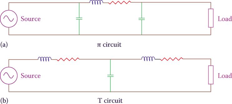
Figure 4 Modeling of transmission lines. (a) π model. (b) T model.