Hysteresis Loop Definition
A curve, or loop, plotted on B-H coordinates showing how the magnetization of a ferromagnetic material varies when subjected to a periodically reversing magnetic field, is known as Hysteresis Loop or Magnetization Curve.
The term ‘hysteresis’ means to lag behind. In electrical terminology it is used to describe the lag between a change in value or direction of the magnetizing force (H) and the resulting change in value or direction of flux (B).
Even after the magnetizing force is removed, some magnetism remains. This is known as residual magnetism. Residual magnetism is that portion of the magnetic flux that remains in a ferromagnetic material when the magnetizing force is removed. In other words, the material remains partially magnetized because it has some permanent magnetic properties.
In order to remove residual magnetism, it is necessary to use a force that acts in the opposite direction to the original magnetizing force. The force that is used to overcome residual magnetism is known as the ‘coercive force ‘the force required to coerce the magnetism from the material.
When a ferromagnetic material is magnetized first in one direction and then in the other, it is necessary to use coercive force to overcome the effect of residual magnetism.
The amount of coercive force required depends on the type of magnetic material. The energy required for the coercive force is wasted and therefore considered to be a loss, resulting in lower efficiency and heating of the magnetic core.
Hysteresis Loop
If the magnetizing force is plotted against the flux density in the classic B/H graph, in both directions the hysteresis can be clearly seen.
Look at Figure 1 and note the initial magnetization curve OA. It begins at the origin (O) when no magnetic force or flux exists, and increases to point A which is well into the saturation region, or past the knee of the curve. The magnetizing force (+ H) results in a flux (+ B) that is saturated.
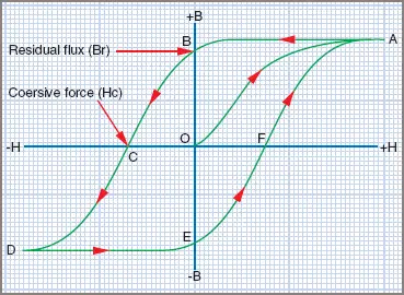
Figure 1 Magnetic Hysteresis Loop
As the magnetizing force is reduced back to zero, the flux density reduces as well, but not to zero. The part of the curve AB represents the removal of the magnetizing force, and the resulting reduction in flux, but point B shows the flux density that remains, the residual flux (Br).
In order to remove the residual magnetism, a reverse magnetizing force is required, called a coercive force (Hc) that causes the flux density to be reduced to zero. Part BC of the curve shows the coercive force in effect.
The negative magnetizing force now continues to increase to point D, which is the maximum negative magnetizing force and a point equal but opposite to point A on both axes.
Curve DEFA is an exact reflection of ABCD. Thus the combined magnetization curves form a closed loop, ABCDEFA. This loop is commonly known as a hysteresis loop for a ferromagnetic material.
OB and OE indicate the values of residual flux density at zero magnetizing force, while the value of the coercive force required to remove that residual flux is indicated by OC and OFAL.
Hysteresis Losses
Reversing the magnetic field requires a coercive force to reverse the residual magnetism, and this requires a current flow. This results in the generation of heat within the magnetic material, which represents a loss of energy, known as hysteresis loss.
How much energy is lost depends on the amount of coercive force required to reverse the magnetic dipoles within the material, and this is directly proportional to the area within the hysteresis loop for that material.
The hysteresis loop determines the suitability of a magnetic material for a particular application. In equipment that is subjected to a rapidly changing flux, it is important that the material used in the magnetic core has a hysteresis loop with a small area.
The maximum height (B) is the designated flux that must be reached, but the width of the loop (H) must be as narrow as possible to reduce losses.
Permanent magnets, however, should require a very large coercive force to be de-magnetized, and therefore the hysteresis loop should be very wide, with a large loop area.
Hysteresis loss appears in the form of heat in the magnetic cores of equipment; these are often iron, particularly in older equipment, and so it is known as ‘iron loss’. Electrical power has to be consumed to make up for iron loss and it is therefore usual to give values of iron loss, for a particular material, in watts per kilogram at a given frequency e.g. 50 Hz.
The area of hysteresis loops obtained from tests on samples of magnetic materials give important information about the suitability of a material for a particular application. Figure 2 compares the hysteresis loops of transformer steel and carbon steel.
It shows that the hysteresis loop for transformer steel is comparatively small in area, which indicates that transformer steel will give a relatively lower iron loss. This is an important factor in the choice of core material for transformers, because rapidly reversing fluxes occur in this application. Carbon steel would not be suitable because of the large iron loss that would occur with this material; however, permanent magnets may be made from carbon steel.
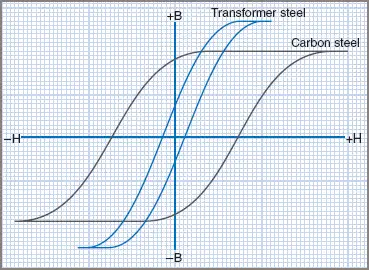
Figure 2 Hysteresis Losses in Materials
Magnetic Leakage and Fringing
In practical magnetic circuits, it is often desirable to have the maximum value of flux in a particular section of the circuit. Unfortunately, the flux tends to spread out, particularly when the flux density is high.
There is a tendency for some of the flux to leak through the surrounding air, bypassing the intended path. Therefore the flux density in the intended path of the magnetic circuit is reduced to a lower value. The magnetizing force must be increased to allow for the losses but, when the core becomes saturated, the amount of energy required to increase the magnetic flux may become uneconomical or even impossible.
Figure 3 illustrates a magnetic circuit for an instrument in which the source of m.m.f. is a strong permanent magnet. In this particular circuit, the maximum possible flux is desirable at the air gap, evenly distributed in the gap between the soft iron pole pieces (A and B) and the armature (C).
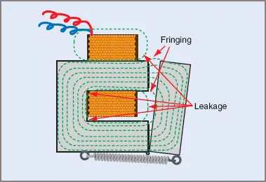
Figure 3 Armature Relay/Contactor Leakage Flux
The total flux of the magnet does not reach the air gap, but leaves the iron poles and passes through the surrounding air. The flux which leaves the main path is known as the leakage flux. The tendency for the leakage flux to stray from the desired path is known as ‘magnetic leakage’. When designing magnetic circuits, engineers allow for magnetic leakage when calculating the values of flux required.
Remember that there are no magnetic insulators, so there is no means of retaining the magnetism within the magnetic conductor.
Figure 3 also shows the magnetic field that exists across an air gap in a magnetic circuit. The lines of force near the center line of the flux path are straight. Lines of force at the edges of the field tend to curve outwards in the air gap and spread according to the rule that flux travelling in like directions repels.
As a result, the area of the flux path is greater in the air gap than in the material of the magnetic circuit. The flux density of the air gap will in consequence be less than that in the magnetic material on either side of the gap. This effect is known as ‘magnetic fringing’ and must be allowed for when designing magnetic circuits in which there are air gaps. Some magnetic leakage also occurs at the sides of the air gap, but this is normally counted as a part of the fringing.