This article explains the static and dynamic characteristics that define sensor performance, including accuracy, sensitivity, resolution, hysteresis, repeatability, response time, and bandwidth. It also discusses how these parameters are specified in datasheets and how they influence measurement reliability and overall system behavior.
Several parameters characterize sensors’ performance. The time-independent characteristics are called the static characteristics, while the time-dependent characteristics are called the dynamic characteristics. The static characteristics characterize the sensor output after it has settled due to changes in the physical quantity being measured. The dynamic characteristics describe the sensor characteristics from the time the physical quantity has changed to the time before the output has settled.
Sensor Static Characteristics
Range
The minimum to maximum value that can be measured is the range. The range defines the allowable range of the physical quantity that can be detected by the sensor.
Accuracy
The difference between the true and actual measured values is the accuracy. It is commonly expressed as a percentage of the full-scale value. For example, if a temperature sensor has a range of 0 to 200°C and an accuracy of +/−0.5% the full-scale value, then the temperature read by the sensor is off from the true actual temperature by +/−1°. Note that accuracy is also referred to as bias, and the accuracy error can be improved by calibration.
Sensitivity
The relationship between the measured input and the output of the sensor is its sensitivity. If the sensor has a linear input–output relationship, then the sensitivity is the slope of this curve. Sometimes, this parameter is used to indicate the sensitivity of the sensor to non-measured input (response due to transverse motion when the sensor is designed to measure axial motion) or the environment (temperature).
Resolution
The smallest change in input value that will produce an observable change in the output is the resolution. The inherent resolution should be distinguished from the display device resolution.
Hysteresis
The maximum difference in sensor output for the same input quantity is the hysteresis, with one measurement taken while the input is increasing from the minimum input and the other by decreasing the input from the maximum input. A sensor with hysteresis will have a different output value that is a function of whether the input quantity was increasing or decreasing when the measurement was made. The hysteresis error is illustrated in Figure 1.
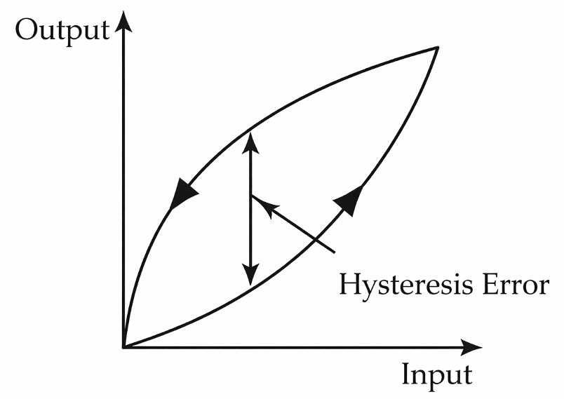
Figure 1. Illustration of hysteresis error
Repeatability
Repeatability refers to the consistency of output values when the same measurement is repeated under identical conditions. The closer the output values are to each other for repeated measurements, the higher the measurement’s repeatability and, by extension, the precision.
Factors like signal interference, vibration, temperature fluctuation, instrument drift, and user variability can introduce variability and affect repeatability. While calibration primarily addresses systematic biases in measurements and does not directly improve repeatability, techniques like taking multiple measurements and using statistical methods can help manage and potentially reduce repeatability errors.
Non-Linearity Error
Most sensors are designed to have a linear output, but their output is not perfectly linear. The nonlinearity error is a measure of the maximum difference between the sensor’s actual output and a straight line fit to the sensor input–output data, and is usually specified as a percentage of the full-scale output. There is no unique way to obtain the straight-line fit. The straight line can connect the minimum and maximum output values that define the sensor range, or it can be obtained from a least-square fit to the entire input–output data or from a least-square fit to the input–output data with one end of the line passing through the origin. Figure 2 illustrates these cases and shows that the magnitude of this error is dependent on how this error is defined.
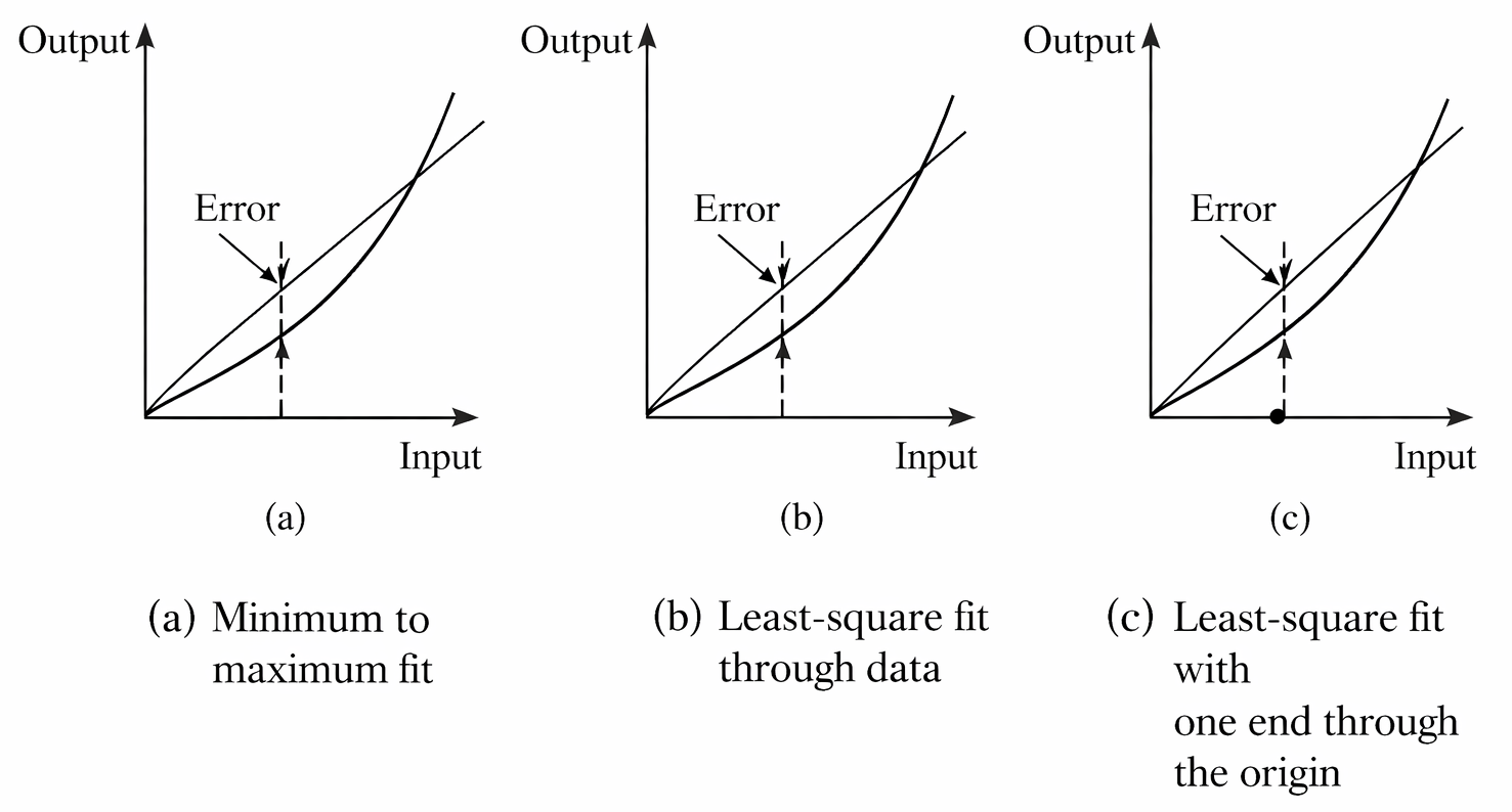
Figure 2. Illustration of nonlinearity error
Stability
Stability or drift refers to the variation of the output with time when the input quantity is not changing. The output variation is called the zero drift when no input is applied to the sensor. Stability affects the repeatability of the measurement.
Sensor Dynamic Characteristics
Rise Time
The time it takes the output to change from 10 to 90% of its final steady-state value is the rise time. It provides a measure of how quickly the sensor output reaches its steady state.
Time Constant
This is defined as the time it takes the output to reach 63.2% of the difference between the final and the initial output. A large time constant implies a sluggish sensor, while one with a small value indicates a rapidly responding sensor.
Settling Time
The time it takes the output to reach within a certain percentage of the final steady–state value is the settling time. A common value is the 2% settling time. The rise time, time constant, and settling time are illustrated in Figure 3 for a sensor with first-order response characteristics.
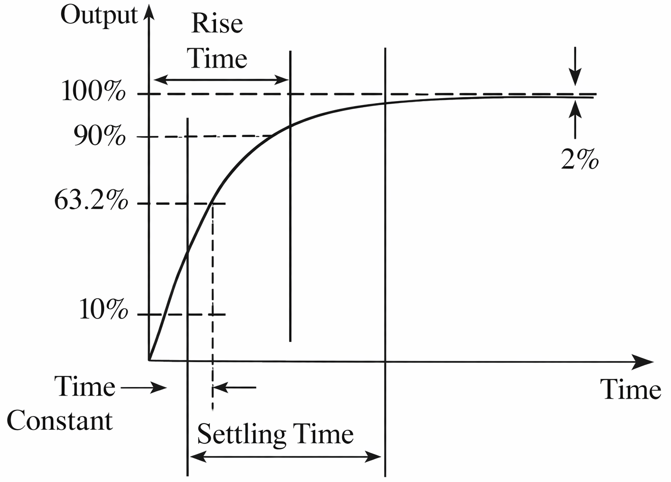
Figure 3. Illustration of basic dynamic response characteristics
Bandwidth
The bandwidth of a sensor defines the frequency range over which it is designed to operate effectively. When utilizing a sensor for feedback in a closed-loop control system, the sensor’s bandwidth needs to exceed that of the controller to ensure that the sensor can accurately measure and relay system responses to the controller without introducing phase lags or distortions that might destabilize the control system.
Values for each sensor performance characteristic are found in the manufacturer’s datasheet for the particular sensor. Normally, the specification in the datasheet is grouped into categories, including dynamic or performance, electrical, mechanical, environmental, and physical. An example of some of the characteristics of a compression load cell is shown in Table 1, including a description of each specification.
Table 1. An Example of the Specifications for a Load Cell Sensor
| Item | Value | Explanation |
| Rated capacity | 10 lbs. | The maximum weight that the cell is rated to handle |
| Excitation | 10 VDC | The cell is designed for an excitation voltage of up to 10 VDC, but it can also operate with lower voltages |
| Rated output | 2 mV/V nominal | The nominal cell output at the rated load (10 lbs) and the maximum excitation voltage (10 V) will be 20 mV (2 mV/V × 10 V) |
| Linearity | +/−0.25% FS | With a 5 lb. load applied, the cell output will indicate a load of 5 lbs. +/−0.025 lb. |
| Hysteresis | +/−0.15% FS | Due to hysteresis, the cell output can vary by +/−0.015 lb. |
| Maximum load (safe overload) | 150% of rated capacity | The cell can handle up to 15 lbs. without risk of damage, but accuracy may be affected |
| Bridge resistance | 350 Ω | The resistance of the strain gauge inside the load cell |
Example 1 illustrates the computation of the maximum error in a sensor measurement.
Example 1: Computation of Total Sensor Error
A linear displacement sensor with a measuring range of 0 to 50 mm has the following specifications: an accuracy of 0.5% of full-scale reading and a linearity error of 0.2% of full-scale reading. Determine the maximum possible error (in mm) one could expect.
Solution
The total error will be the sum of the accuracy error and the linearity error.
The accuracy error = accuracy (as %) × full-scale reading/100 = 0.5 × 50/100 = 0.25 mm.
The linearity error = linearity error (as %) × full-scale reading/100 = 0.2 × 50/100 = 0.1 mm.
Summing the two errors (0.25 + 0.1) gives the total error as 0.35 mm. This is the maximum possible error when taking a reading with this displacement sensor.
This solution assumes that all the sources of error are additive, which represents a worst-case scenario. This assumption often provides a conservative estimate of error that ensures safety and robustness in various applications, particularly in engineering. Some errors might be systematic (always in one direction) while others might be random. In such cases, the errors might not necessarily add up to a worst-case scenario.
Key Takeaways
Understanding sensor static and dynamic characteristics is essential for selecting and applying sensors in real-world engineering systems. These parameters directly affect measurement accuracy, control system stability, safety margins, and long-term reliability in applications ranging from industrial automation and robotics to automotive systems and biomedical instrumentation. Careful interpretation of datasheet specifications—along with awareness of error sources, response limits, and environmental influences—ensures that sensors are properly matched to their intended operating conditions.