Impulse Response due to Real and Complex Poles | Matlab

Time Response due to Distinct Poles

In addition to computing the time response of the output, we can use MATLAB to evaluate and display the time response due to an individual real pole or to a pair of complex poles. Recall that a real pole at s = p with residue r will result in the time function

$y(t)=r{{e}^{pt}} $  for t>0.

 If a pole is complex, say at s₁=σ+jω, then its complex conjugate s₂=σ+jω will also be a pole. The residue at s₁ will be a complex number, say ${{r}_{1}}=K{{e}^{j\phi }}$, and the residue at s₂ will be the complex conjugate of r₁, namely, ${{r}_{2}}=K{{e}^{-j\phi }}$. It can be shown that for t>0 the time response due to this pair of complex poles is

$y(t)=2K{{e}^{\sigma t}}\cos (\omega t+\phi )$

To simplify the calculation of these responses, we have created two functions designated as named rpole2t and cpole2t. The former has as its arguments the value of the real pole, its residue, and a time vector. The function returns a column vector of time response values, one per time point. The latter function has the value of the complex pole with the positive imaginary part as its first argument, the residue at this pole as the second argument, and a time vector as the final argument.

Impulse Response due to Real and Complex Poles Matlab Example

Use the poles and residues of the transfer function G(s) to display the components of g(t) due to the real pole at s = -0.2408 and the complex poles at s = -0.8796 1± j1.1414. Verify that the sum of these two responses equals the impulse response shown in tutorial 2.

\[\begin{matrix}   G(s)=\frac{3s+2}{2{{s}^{3}}+4{{s}^{2}}+5s+1} & \cdots  & (1)  \\\end{matrix}\]

We can write the partial-fraction expansion of the transfer function as

\[\begin{matrix}   G(s)=\frac{0.3734}{s+0.2408}+\frac{-0.1867-j0.5526}{s+0.8796-j1.1414}+\frac{-0.1867+j0.5526}{s+0.8796+j1.1414} & \cdots  & (2)  \\\end{matrix}\]

Solution

Referring to Table 1 in tutorial 2,

Table.1: Poles and residues of G(s)

Pole	Residue
-0.2408	0.3734
-0.8796 +j1.1414	-0.1867 -j0.5526
-0.8796 -j1.1414	-0.1867 + j0.5526

 We use the function rpole2t with the pole s = -0.2408 and the residue r = 0.3734 to obtain the response due to the one real pole of G(s). The resulting time function is the inverse Laplace transform of the first term of G(s). For the other two terms in (2), which result from the complex poles, we use the pole having the positive imaginary part, namely s = -0.8796 + j 1.1414 and its residue r = -0.1867 – j0.5526. The MATLAB instructions that will accomplish these steps and plot the responses are shown in Script 3, and the resulting responses are shown in Figure 1.

Matlab Code for Calculating Impulse Response

% Script 3: Impuse Response due to rel and complex poles

clear all;close all;clc

numG = [3 2]; denG = [2 4 5 1]; % create G(s) as ratio of polys

[resG,polG,otherG] = residue(numG,denG) % residues & poles of G(s)from equation (1)

t = [0:0.1:20]; % column vector of time points

ycmplx = cpole2t(polG(1),resG(1),t); % response due to complex pole

yreal = rpole2t(polG(3),resG(3),t); % response due to real pole

ytot = ycmplx + yreal; % y(t) is sum of the two

plot(t,ytot,t,ycmplx,t,yreal,'--') % plot the three curves

Function rpole2t

function y_out = rpole2t(real_p,residue,time)
% This function computes Inverse Laplace Transformation
%for a real pole in order to generatea time function
%Inputs for this function are:
%real_p - real pole
% residue - residue at the real pole
% time - a time vector
% That's how we compute the response as
 % y(t) = residue * exp(real_p*t) 
y_out = 0*time;
for t=1:length(time),
 y_out(t) = residue*exp(real_p*time(t));
end
y_out = real(y_out);
%%%%%%%%%%

Function cpole2t

function y_out = cpole2t(comp_p,residue,time)
% This function computes Inverse Laplace Transformation
%for two complex conjugate poles in order to generate a time function
% 
%Inputs for this function are:
%comp_p - complex poles with Positive Imaginary Parts
% residue - residue at the complex pole
% time - a time vector
%Output: 
%y_out - indicates time response vector as an output
% 
% That's how we compute the response 
% y(t) = 2*K*exp(m*t)*cos(Omega*t + phii)
% where residue = K*exp(j*phii), comp_p = m + j*Omega

m = real(comp_p); % Pole zero component
Omega = imag(comp_p); % Pole imaginary component
K = abs(residue); % to compute absolute value
phii = angle(residue); % to compute angle phii
y_out = 0*time;
for t=1:length(time),
 y_out(t) = 2*K*exp(m*time(t))*cos(Omega*time(t)+phii);
end
y_out = real(y_out);
%%%%%%%%%%

Result

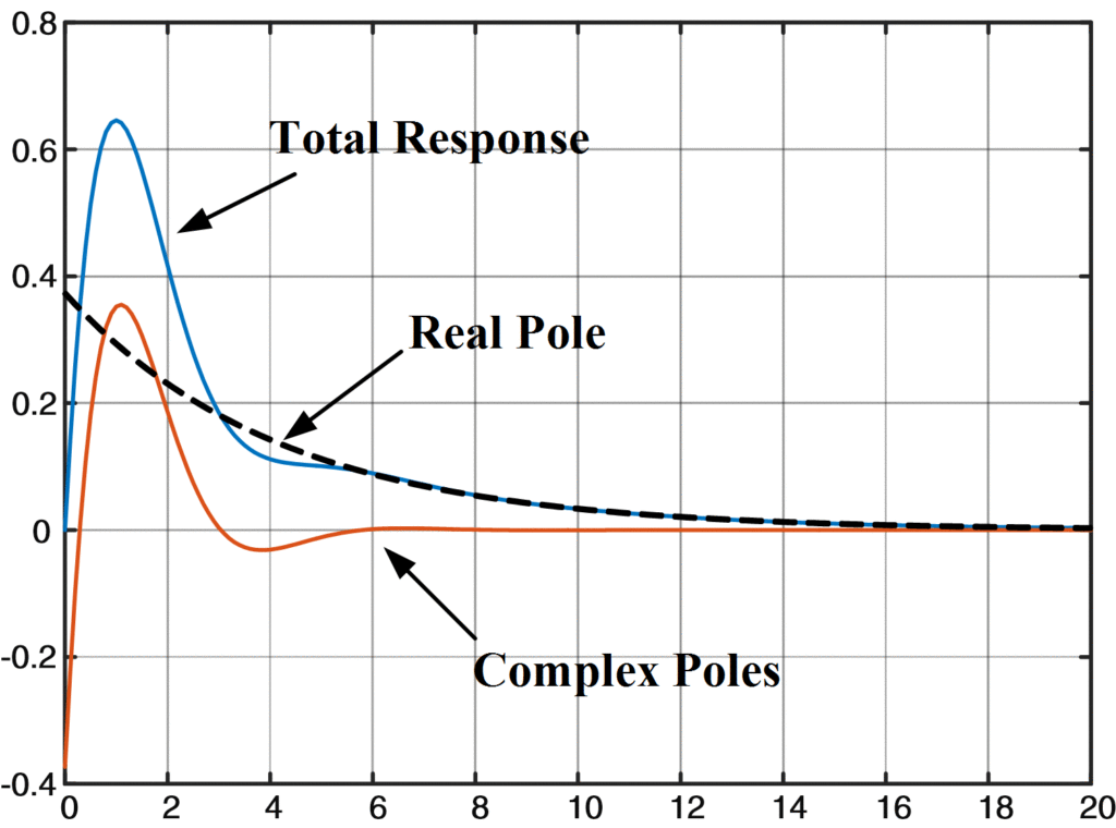
Fig.1: Impulse Response for Real and Complex Poles

So, from the graph, it’s evident that the “Total Response” here is the same as we obtained in tutorial 2.