Step Response
The Laplace transform of a system’s unit step response is the product of the system’s transfer function G(s), and 1/s, the transform of the unit step function. The poles of the resulting transform are the poles of G(s) and a pole at s = 0 (due to the unit—step input). The zeros and gain of the step response are the same as those of the transfer function. The step response can be computed and plotted using the step command from the Control System Toolbox. This command has the same options as does the impulse command for plotting and returning numerical values.
DC Gain of a Transfer Function
The gain at s = 0 is G(0) and is known as the DC gain. It is the ratio of the constant terms in the numerator and denominator polynomials. We can compute the DC gain directly from the TF form using the Control System Toolbox command dcgain (num, den).
In the following example, we use MATLAB to construct the Laplace transform of a step response, plot the response with the impulse command, and compare the result with a plot obtained using the step command. We also illustrate the use of the initial- and final-value theorems.
Step response using Matlab Example
For the transfer function G(s)
\[G(s)=\frac{3s+2}{2{{s}^{3}}+4{{s}^{2}}+5s+1}\]
Obtain a plot of the step response by adding a pole at s = 0 to G(s) and using the impulse command to plot the inverse Laplace transform. Compare the response with that obtained with the step command applied to G(s). Also, determine the system’s DC gain. Use the initial- and final—value theorems to check your results.
Solution
To add a pole at s = 0, we multiply the denominator polynomial by s. In MATLAB, this can be done in either of two ways.
Add Pole to Transfer Function
One method is to use the “conv” command, which will multiply two polynomials by performing a discrete convolution of the row vectors containing their coefficients. In this example, we want to multiply the denominator of G(s) by the polynomial s, which in MATLAB is represented by the row vector [1 0]. To do this, we enter denstep= conv (denG,[1 0]).
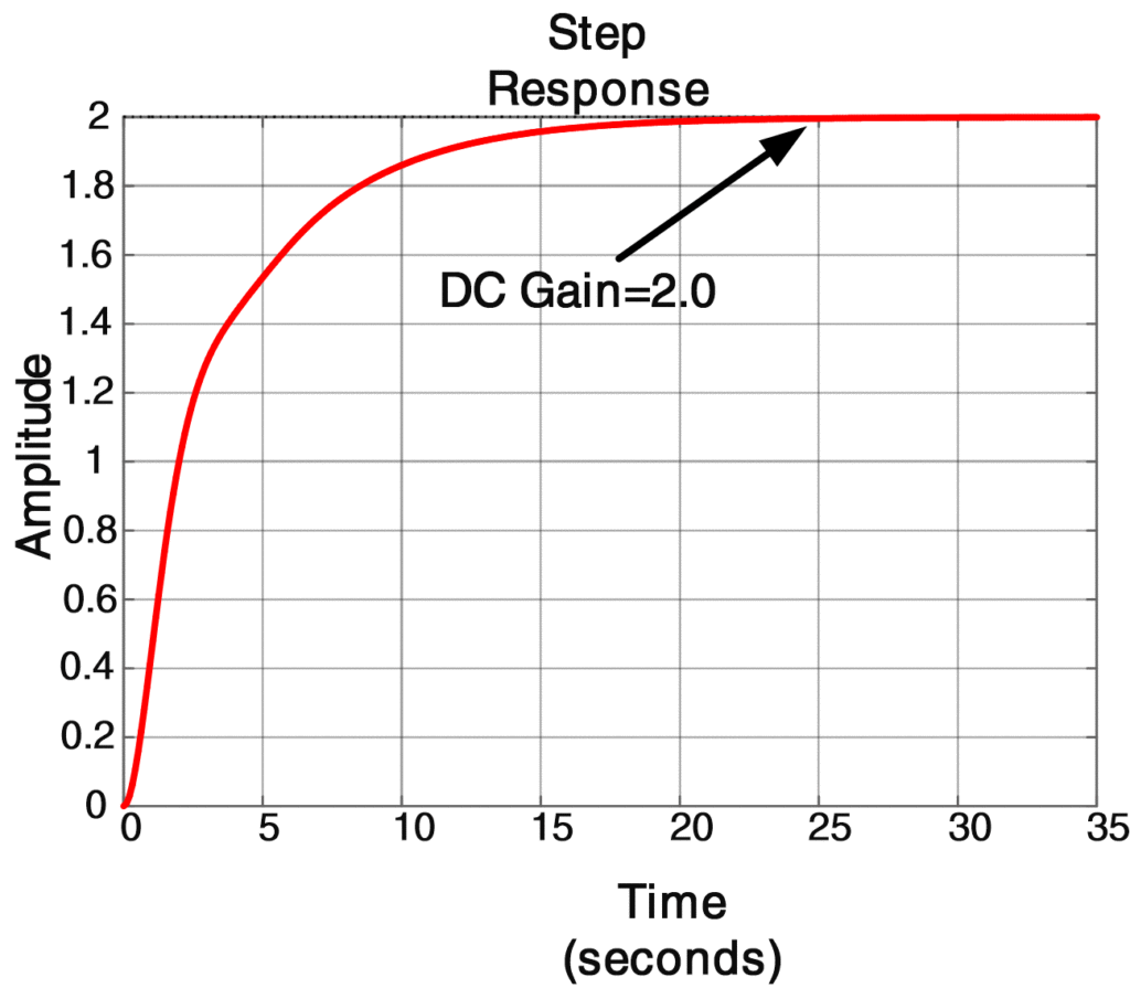
The other method is to append a 0 to the row vector denG with the statement denstep = [denG 0]. The numerator of the transform of the step response is the same as that of G(s), so we write numstep = numG. Having obtained the transform of the unit step response in terms of the row vectors numstep and denstep, we use the impulse command to get the inverse transform, which is the step response shown in Figure 1. Alternatively, we could have used the transfer function G(s) as expressed by the polynomials numG and denG and the step command to generate the same plot. The calculation of the DC gain gives a value of 2.0, which agrees with G (0) as obtained by letting s = 0 in (1). These commands are contained in Script 5.
Matlab Code to Calculate and Plot Step Response
%Script 5: Matlab Code for Step Response from G(s)

clear all;close all;clc

numG=[3 2]; denG=[2 4 5 1]; % create G(s) as ratio of numerator & Denumerator

numstep=numG; % no change to numerator

denstep=[denG 0]; % add pole at s=0 to G(s)

%A plot of the step response by adding a pole at s = 0

%to G(s) and using the IMPULSE command

impulse(numstep,denstep)

% A plot of the step response using STEP command applied to G(s)

step(numG,denG,'r')

% Calcualte G(0) from TF Form

dcgain(numG,denG)
Result

Fig.1: Step Response using Matlab Transfer Function
Note: As mentioned in the text, both IMPULSE and STEP commands produce the same plot. This can be checked by commenting one command at a time and obtain the response plot.
If ys(t) denotes the system’s unit step response, we can see from figure 1 that ys(0+)=0 and ys(∞)=2. To verify these values analytically, we write the Laplace transform of the step response as
$Ys(s)=\frac{1}{s}G(s)=\frac{3s+2}{2(2{{s}^{3}}+4{{s}^{2}}+5s+1)}$
The initial-value theorem gives
${{y}_{s}}(0+)=\underset{s\to \infty }{\mathop{\lim }}\,s{{Y}_{s}}(s)=\underset{x\to \infty }{\mathop{\lim }}\,\frac{3s+2}{2{{s}^{3}}+4{{s}^{2}}+5s+1}=0$
And the final-value theorem gives
${{y}_{s}}(\infty )=\underset{s\to 0}{\mathop{\lim }}\,s{{Y}_{s}}(s)=\underset{x\to 0}{\mathop{\lim }}\,\frac{3s+2}{2{{s}^{3}}+4{{s}^{2}}+5s+1}=2$
As an option, you can delegate your assignment to experts and get MATLAB homework help online here – at AssignmentCore.