Zero State Response using Matlab

Response to a General Input

In addition to computing and plotting the impulse and step responses of a system, MATLAB can be used to find and display the response to general functions of time. This is done with the lsim command, which can be used in a variety of ways. In its simplest form, the user specifies the system’s transfer function, a vector of input values, and a vector of time points.

lsim Matlab Command

If the lsim command, which performs linear simulation, is given with no output variable, the plot of the response is drawn but no numerical values are returned.

A more useful way to use this command is to specify the system output (y) as a result and then to plot both the output and the input (u) versus time. We illustrate the use of lsim in the following example by solving for the zero-state response to an input signal that is piecewise constant.

Zero State Response using Matlab Example

Find the zero-state response of the system G(s) to the input u (t)

\[G(s)=\frac{3s+2}{2{{s}^{3}}+4{{s}^{2}}+5s+1}\]

\[u(t)=\left\{ \begin{matrix}   \begin{matrix}   0 & t<0  \\\end{matrix}  \\   \begin{matrix}   2 & 0\le t<2  \\\end{matrix}  \\   \begin{matrix}   0.5 & t\ge 2  \\\end{matrix}  \\\end{matrix} \right.\]

Solution

Once the system’s transfer function has been defined by creating the vector of polynomial coefficients numG and denG, we need to create vectors of time points and input values. The only constraints are that the time points must be uniformly spaced and that the two vectors must have the same number of elements. We start by defining time to be a column vector that has a sufficiently small time increment (say, 0.02 s) to yield a smooth response plot and a large enough maximum time to show all of the transients. The command time = [0:0.02:10] ‘ will accomplish this for the system and input signal under consideration.

The input vector u can be created in a number of ways. As shown in Script 6, we first use the ones command to make u be a vector having the same dimension as time but with all of its values equal to 2.0.Then we use a for loop to change the values of all the elements corresponding to t≥2 from 2.0 to 0.5. Note that the range of the index i for which the values are changed is calculated by MATLAB based on the properties of time and u by using the commands min, find, and length. Specifically, min (find (time>=2. 0)) is the index of the first time point that is greater or equal to 2.0 s. This is because find (time>=2. 0) returns the indices of all the time points that are 2.0 or greater, and the min function selects the smallest of these. Also, length (u) is the index of the last element of the input vector u. This approach has the advantages that one does not have to calculate the starting and ending values of the index i and that no modifications are required if the number of time points is subsequently changed, due to a change in either the time increment or the maximum time.

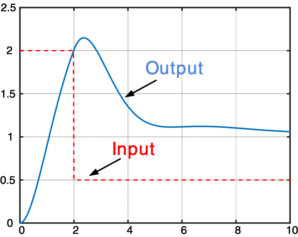
The values of the response are computed by the command lsim and are stored in the column vector y. Then both y and u are plotted versus time, resulting in Figure.

Matlab Code to Compute Zero-Response using lsim 

%Script 6: Matlab Code to compute Zero-Response

clear all;close all;clc

numG = [3 2]; denG = [2 4 5 1]; % create G(s) as ratio of numerator & denumerator

time = [0:0.02:10]; % 501 time points, every 0.02 s

u = 2.0*ones(size(time)); % construct 501 input values

%Here, min (find (time>=2. 0)) is the index of the first time point

%that is greater or equal to 2.0 s. This is because find (time>=2. 0)

%returns the indices of all the time points that are 2.0 or greater,

%and the min function selects the smallest of these.

%also, length (u) is the index of the last element

%of the input vector u

for i=min(find(time>=2.0)):length(u) % start with all points = 1.0

u(i) = 0.5; % then change to 0.5 if t>=2.0

end

%lsim command performs linear simulation to compute the response

%For more understanding, write "help islm" in Maltab Command Window

y = lsim(numG,denG,u,time);

% Plotting the input & Output Response

plot(time,y,time,u,'--')

Result

Fig.1: Zero State Response using Matlab Example