This article introduces the Z-transform, a tool for analyzing discrete-time linear time-invariant systems, and discusses its properties, including linearity, time shifting, scaling, time reversal, differentiation, and convolution. It also explains the importance of the region of convergence (ROC) in determining system stability and sequence characteristics, and covers key theorems such as the initial and final value theorems.
INTRODUCTION TO Z-TRANSFORM
For the sake of analyzing continuous-time linear time-invariant (LTI) system, Laplace transformation is utilized. And z-transform is applied for the analysis of discrete-time LTI system. Z-transform is fundamentally a numerical tool applied for a transition of a time domain into frequency domain and is a mathematical function of the complex-valued variable named Z. The z-transforms of any discrete time signal x (n) referred by X (z) is specified as
$X\left( z \right)=\sum\limits_{n=-\infty }^{\infty }{x\left[ n \right]{{z}^{-n}}}$
Z transform is a non-finite power series as summing index number n changes from -∞ to ∞. However, it is valuable for values of z for which aggregate is finite (bounded). The values of z for which function f (z) is finite and lie down inside the region named as “region of convergence (ROC)”.
Merits OF Z-TRANSFORM
- The discrete Fourier transform (DFT) can be computed by assessing z-transform.
- Z-transform is extensively applied for analysis and synthesis of several types of digital filters.
- Z-transform is utilized in many applications such as linear filtering, finding linear convolution, and cross-correlation various sequences.
- System can be characterized (like stable/unstable, causal/anti-causal) using z-transform.
Merits OF REGION OF CONVERGENCE (ROC)
- It, in fact, decides whether given system is stable or not.
- It determines the character of sequences whether causal or anti-causal.
- It likewise determines finite or infinite length sequences.
Z-TRANSFORM PLOT
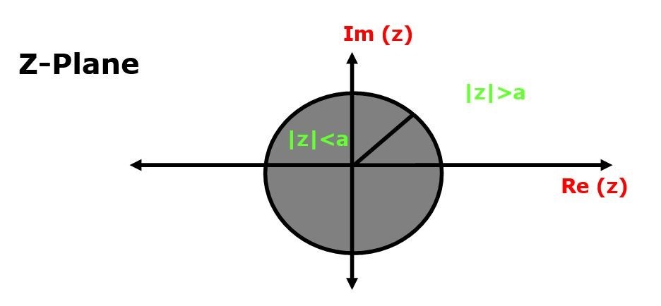
Above figure displays the diagram of z-transform with the region of convergence (ROC). The z-transforms possesses both real and imaginary components. Therefore a diagram of the imaginary component against real component is titled complex z-plane. The radius of the above circle is 1 so named as unit circle. The complex z plane is utilized to demonstrate ROC, poles, and zeros of a function. Complex variable z is carried in terms of polar form as
\[Z=\text{ }r{{e}^{j\omega }}\]
Whereas r is the radius of a circle, and ω is the angular frequency of the given sequence.
Z-TRANSFORM PROPERTIES
1) Linearity
The linearity property describes that if
${{x}_{1}}[n]\overset{z}\leftrightarrows{{X}_{1}}(z)$ and
${{x}_{2}}[n]\overset{z}\leftrightarrows{{X}_{2}}(z)$
then
\[{{a}_{1}}{{x}_{1}}\left[ n \right]\text{ }+\text{ }{{a}_{2}}{{x}_{2}}\left[ n \right]~~\overset{z}\leftrightarrows~~{{a}_{1}}{{X}_{1}}\left( z \right)\text{ }+\text{ }{{a}_{2}}{{X}_{2}}\left( z \right)\]
From preceding relation, we can infer that Z-Transform of a linear combination of two signals is equal to the linear combination of z-transform of two separate signals.
2) Time shifting
The Time shifting property describes that if
\[x\left[ n \right]~~~\overset{z}\leftrightarrows~~~X\text{ }\left( z \right)\] then
\[x\text{ }\left[ n-k \right]~~~~~~~\overset{z}\leftrightarrows~~~~~~X\text{ }\left( z \right)\text{ }{{z}^{-k}}\]
From above, it’s obvious that transferring the sequence circularly by ‘k’ number of samples is equal to multiplying its z-transform by z-k element.
3) Scaling
This property describes that if
\[x\left[ n \right]~~~\overset{z}\leftrightarrows~~~X\text{ }\left( z \right)\] then\[{{a}^{n}}~~x\left[ n \right]\overset{z}\leftrightarrows~X\text{ }\left( z/a \right)\]
So, we can say that scaling the function in z-transform is equal to multiplying it by factor an in time domain.
4) Time reversal Property
The Time reversal property describes that if
\[x\left[ n \right]~~~\overset{z}\leftrightarrows~~~X\text{ }\left( z \right)\] then
\[~x\text{ }\left[ -n \right]~~~~~~~~~\overset{z}\leftrightarrows~~~~~~~~X\text{ }\left( {{z}^{-1}} \right)\]
It implies that if the certain sequence is folded then in z domain, it is just equal to substituting z by z-1.
5) Differentiation in z-domain
The Differentiation property describes that if
\[x\left[ n \right]~~~\overset{z}\leftrightarrows~~~X\text{ }\left( z \right)\] then
\[~n\text{ }x\text{ }\left[ n \right]~\overset{z}\leftrightarrows~-z\text{ }\frac{d\left( X\text{ }\left( z \right) \right)}{dx}\]
6) Convolution Theorem
The Circular property describes that if
${{x}_{1}}[n]\overset{z}\leftrightarrows{{X}_{1}}(z)$ and
${{x}_{2}}[n]\overset{z}\leftrightarrows{{X}_{2}}(z)$ then
\[{{x}_{1}}\left[ n \right]\text{ }*\text{ }{{x}_{2}}\left[ n \right]~\overset{z}\leftrightarrows~{{X}_{1}}\left( z \right)\text{ }{{X}_{2}}\left( z \right)\]
Convolution of two sequences in time domain equates to a multiplication of Z transform of both sequences.
7) Correlation Property
The Correlation of two sequences describes that if
${{x}_{1}}[n]\overset{z}\leftrightarrows{{X}_{1}}(z)$ and
${{x}_{2}}[n]\overset{z}\leftrightarrows{{X}_{2}}(z)$ then
\[\sum\limits_{n=-\infty }^{\infty }{{{x}_{1}}\left( n \right)~{{x}_{2}}\left( -n \right)~}~~~~\overset{z}\leftrightarrows~~~~~{{X}_{1}}\left( z \right)\text{ }{{X}_{2}}\left( {{z}^{-1}} \right)\]
8) Initial value Theorem
Initial value theorem describes that if
\[x\left[ n \right]~\overset{z}\leftrightarrows~X\text{ }\left( z \right)\] then
\[x\text{ }\left[ 0 \right]~~=~{{\lim }_{z\to \infty }}\text{ }X\left( z \right)\]
9) Final value Theorem
Final value theorem describes that if
\[x\left[ n \right]~~~\overset{z}\leftrightarrows~~~X\text{ }\left( z \right)\] then
\[{{\lim }_{n\to \infty }}\text{ }x\left[ n \right]~=\text{ }{{\lim }_{z\to 1\text{ }}}\left( z-1 \right)\text{ }X\left( z \right)~\]
Z Transform Introduction Key Takeaways
The Z-transform is a fundamental tool in the analysis and design of discrete-time linear time-invariant systems. Its various properties, including linearity, time shifting, scaling, time reversal, differentiation, and convolution, offer a comprehensive framework for manipulating and understanding discrete signals. The region of convergence (ROC) is crucial in determining the stability of a system and the nature of its sequences, while key theorems such as the initial and final value theorems help predict the system’s behavior at specific time instances. These properties and theorems have wide-ranging applications in fields like digital signal processing, communication systems, and control theory, where they are essential for designing filters, analyzing system stability, and performing tasks like linear filtering and convolution.