Continuous Time Graphical Convolution Example

This is the continuation of the PREVIOUS TUTORIAL.

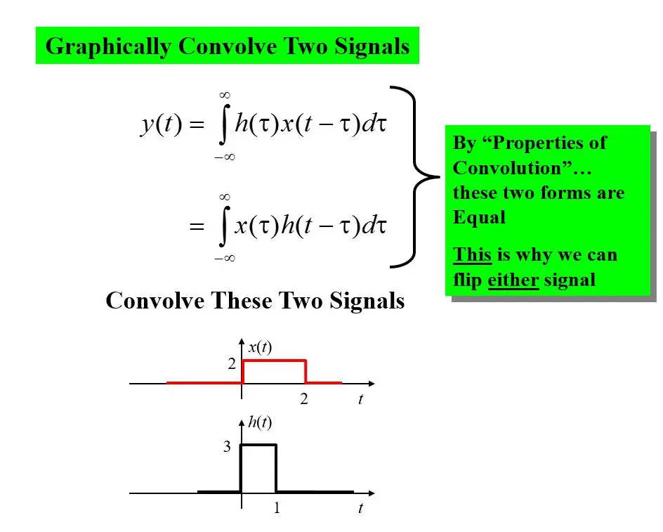
Steps for Graphical Convolution

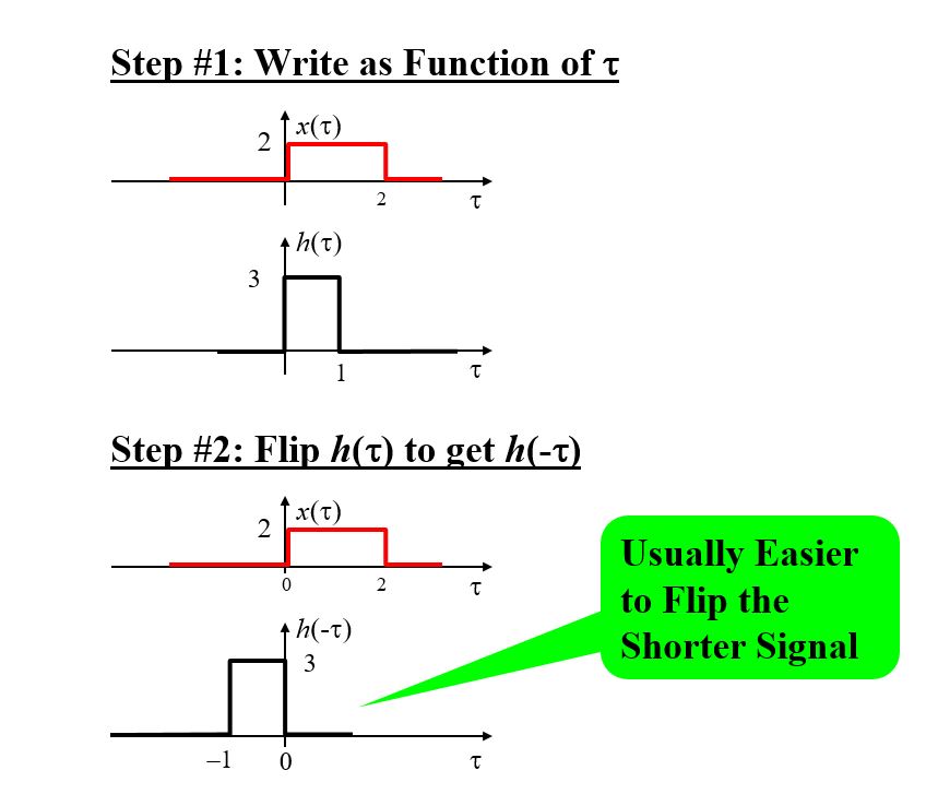
1. First of all re-write the signals as functions of τ: x(τ) and h(τ)

2. Flip one of the signals around t = 0 to get either x(-τ) or h(-τ)

• Best practice is to flip the signal with shorter interval
• We will flip h(τ) to get h(-τ) throughout the steps

3. Determine Edges of the flipped signal

• Determine the left-hand edge τ-value of h(-τ): say τ_L,0
• Determine the right-hand edge τ-value of h(-τ): say τ_R,0

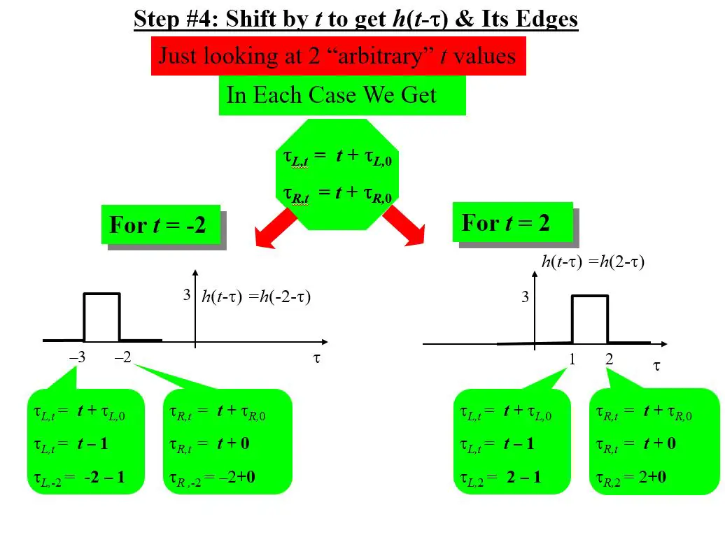
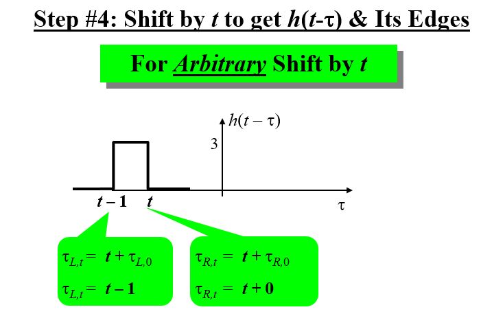
4. Shifting h(-τ) by a random value of t to obtain h(t-τ) and get its edges

• Determine the left-hand edge τ-value of h(t-τ) as a function of t: say τ_L,t

        Noteworthy: It will forever be…τ_L,t = t + τ_L,0

• Determine the right-hand edge τ-value of h(t-τ) as a function of t: say τ_R,t

        Noteworthy: It will forever be…τ_R,t = t + τ_R,0

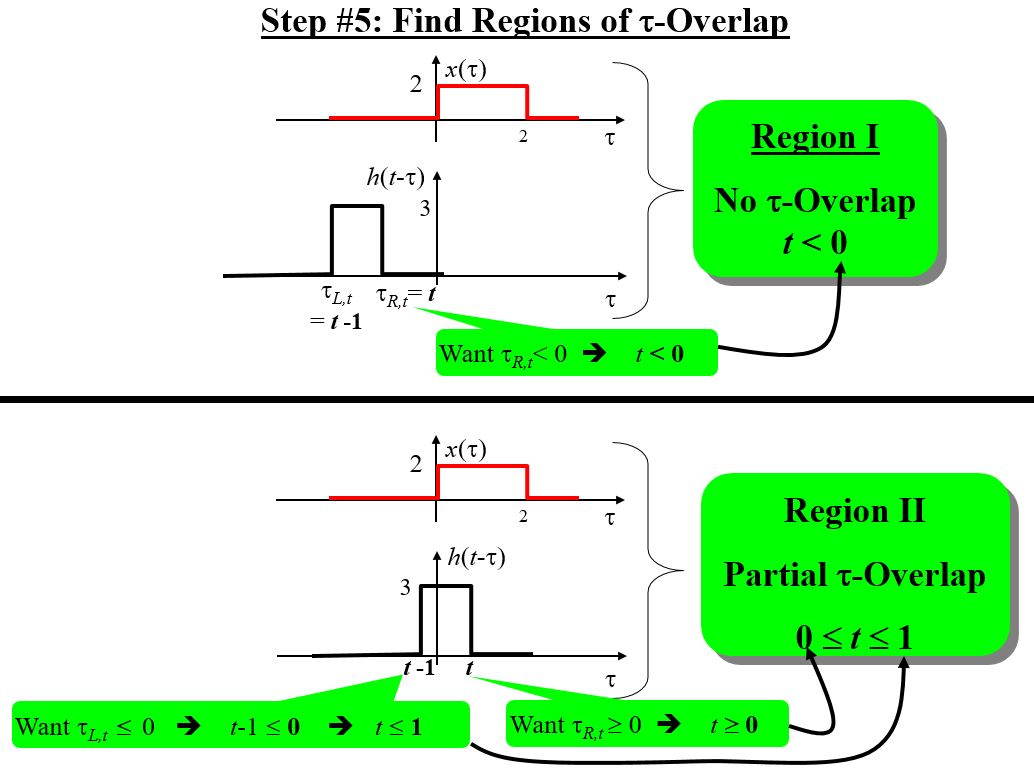
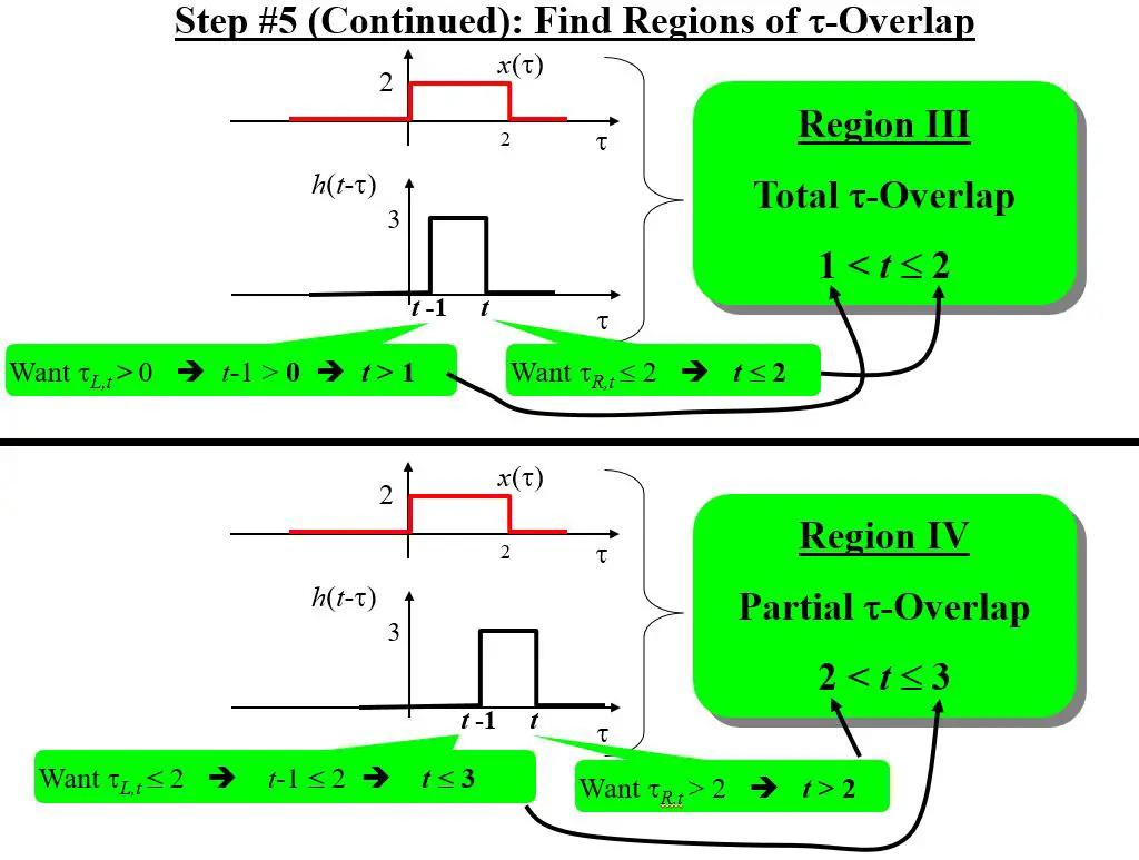
5. Find out Regions of τ-Overlap

•  Determine intervals of t over which the product x(τ) h(t-τ) possesses a single unique mathematical form in terms of τ

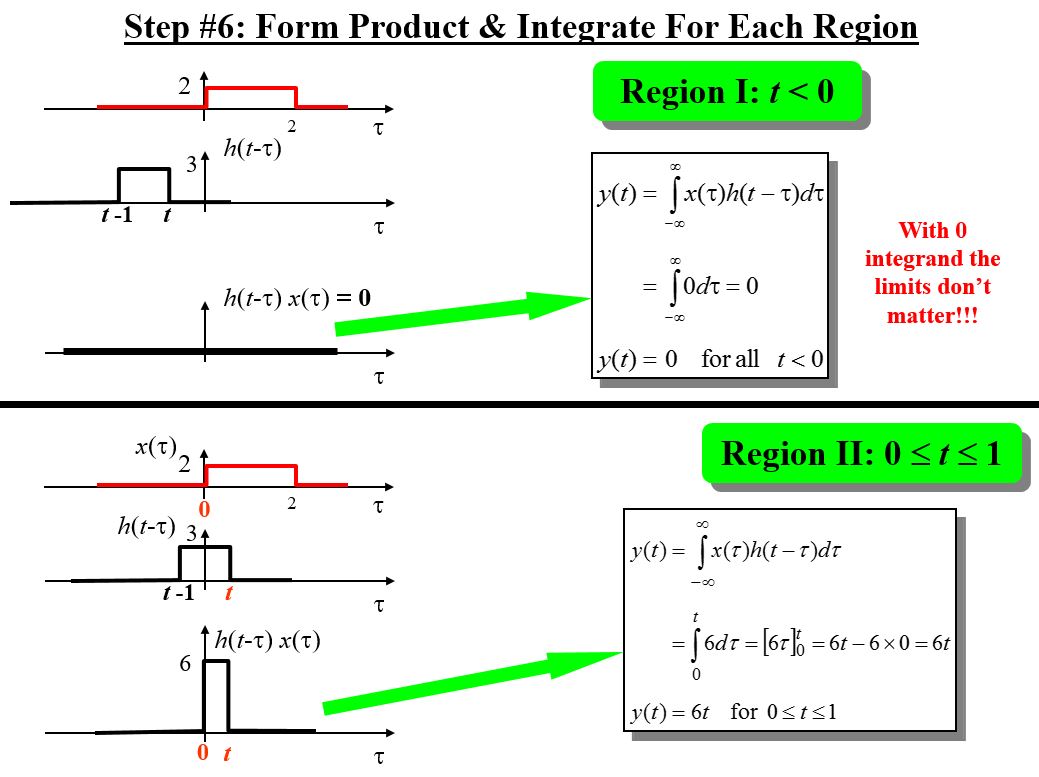
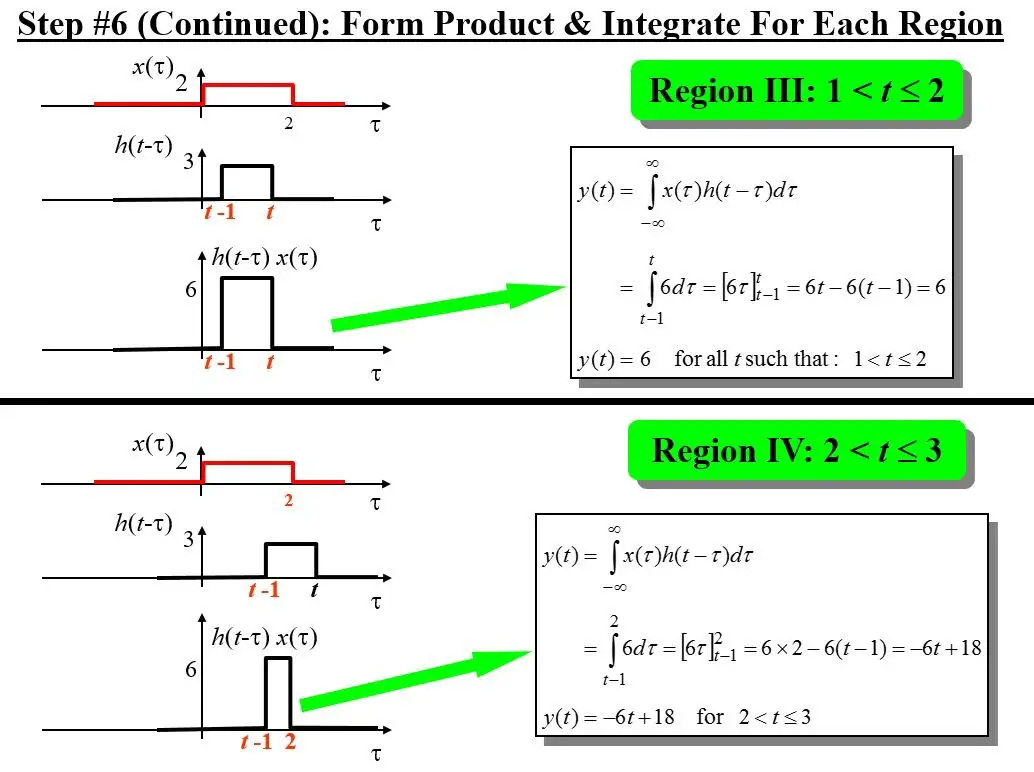
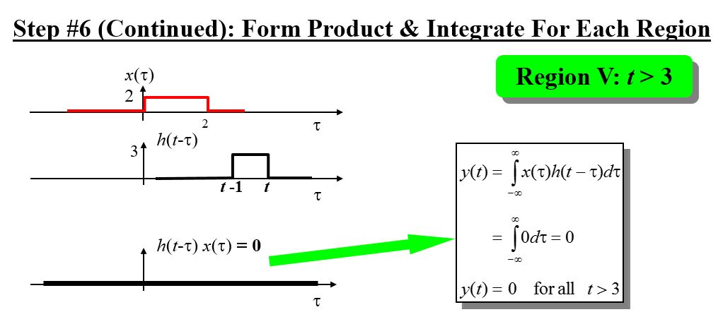
6. For Each Particular Region: develop the Product x(τ) h(t-τ) and Integrate

• Develop the product x(τ) h(t-τ)

• Determine the boundaries of Integration by determining the interval of τ over which the mathematical product is nonzero

•  Determine by discovering where the bounds of x(τ) and h(t-τ) lie down
•  Call back that the bounds of h(t-τ) are τ_L,t and τ_R,t , which frequently depend upon the value of t

• Integrate the product x(τ) h(t-τ) over the boundaries determined in 6b

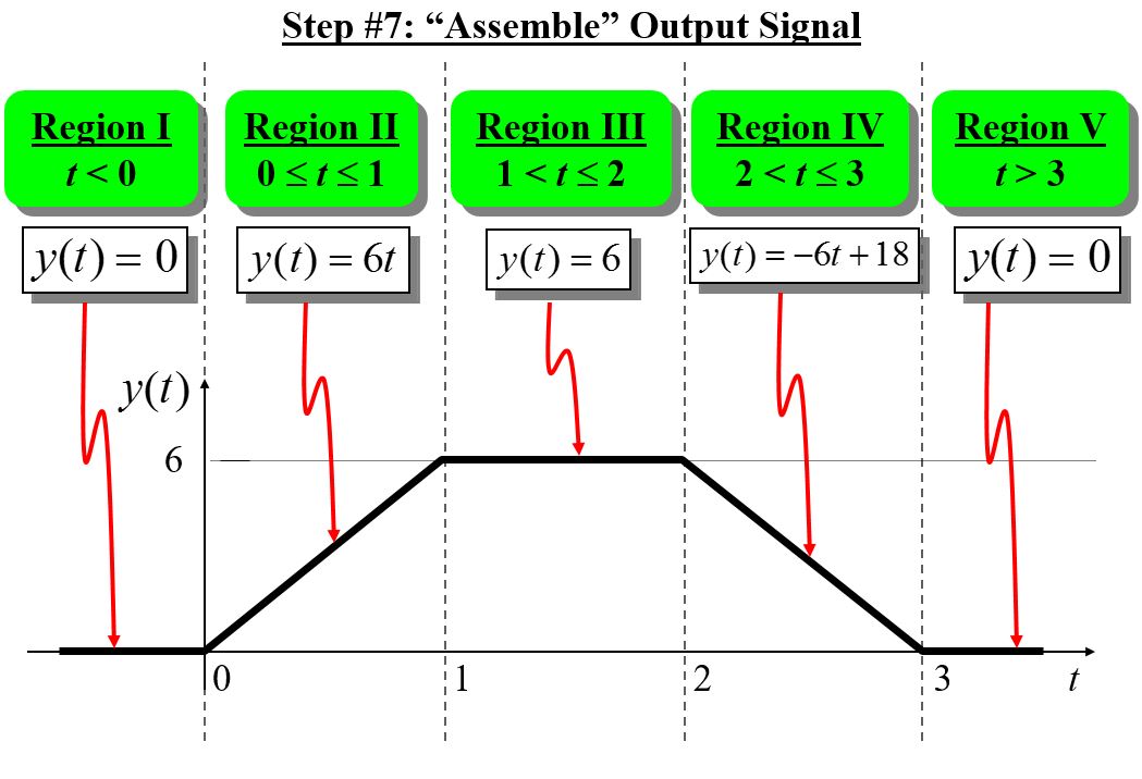
7. “Put Together” the output from the output time-sections for each of the region important:

• DO NOT add together all the sections

• Specify the output in “piecewise” manner

This example is provided in collaboration with Prof. Mark L. Fowler, Binghamton University.

• You May Also Read: Continuous-Time Convolution Properties