Laplace Transform:Introduction and Example

This article introduces the concept of the Laplace transform, its definition, and its applications in analyzing continuous-time functions. It also explores the conditions for the existence of the transform, the region of absolute convergence, and provides an example using the unit step function to demonstrate the Laplace transform’s calculation and behavior.

Laplace Transform Definition

The Laplace transform X(s) is a complex-valued function of the complex variable s. In other words, given a complex number s, the value X(s) of the transform at the point s is, in general, a complex number.

Given a function x (t) of the continuous-time variable t, the two-sided Laplace transform of x (t), denoted by X(s), is a function of the complex variable s=σ+jω defined by

                                         \[X(s)=\int_{-\infty }^{\infty }{x(t){{e}^{-st}}dt}\text{         }(1)\]  

The one-sided Laplace transform of x (t), also denoted by X(s), is defined by

                                            \[X(s)=\int_{0}^{\infty }{x(t){{e}^{-st}}dt}\text{               (2)}\]

By (2), we see that one-sided transform depends only on the values of the signal x (t) for t≥0. This is the reason that definition (2) of the transform is called the one-sided Laplace transform. We can apply the one-sided Laplace transform to signals x (t) that are nonzero for t<0; however, any nonzero values of x (t) for t<0 will not be recomputable from the one-sided transform.

• You May Also Read: Laplace Transform Properties 

If x (t) is zero for all t<0, the expression (1) reduces to (2), and thus, in this case, the one-sided and two-sided transforms are the same. Let Λ denote the set of all positive or negative real numbers σ such that

                 \[X(s)=\int_{0}^{\infty }{\left| x(t) \right|{{e}^{-\sigma t}}dt}<\infty \text{                  (3)}\]

If the set Λ is empty, that is, there is no real number σ such that (3) is satisfied, the function x (t) does not have a Laplace transform (which converges “absolutely”). Most functions arising in engineering do have a Laplace transform, and thus the set Λ is not empty in many cases of interest.

If Λ is not empty, let σ_min denote the minimal element of the set Λ; that is, σ_min is the smallest number such that

σϵ Λ          for all  σ> σ_min

The set of all complex numbers s such that

      _{\[Real\text{ }s>{{\sigma }_{min}}\text{             (4)}\]}    

Where Real s = real part of s, is called the region of absolute convergence of the Laplace transform of x (t). for any complex number s such that (4) is satisfied, the integral in (2) exists, and thus the Laplace transforms X(s) exists for this values of s. Hence the Laplace transform X (s) of x (t) is well defined for all values of s belonging to the region of absolute convergence. It should be stressed that the region of absolute convergence depends on the given function x (t).

Laplace Transform Example

Suppose that x (t) is the unit step function u(t). then the Laplace transform U (s) of u (t) is given by

\[U(s)=\int\limits_{0}^{\infty }{u(t){{e}^{-st}}dt}\]

                                                            \[=\int\limits_{0}^{\infty }{{{e}^{-st}}dt}\]

                                        \[=-\frac{1}{s}\left. {{e}^{-st}} \right]_{t=0}^{t=\infty }\text{                 (5)}\]

Now exp (-st) evaluated at t=∞ is defined by

            \[{{e}^{-s\infty }}=\underset{T\to \infty }{\mathop{\lim }}\,{{e}^{-sT}}\text{                   (6)}\]

Setting s=σ+jω in the right side of (6), we have

                      \[{{e}^{-s\infty }}=\underset{T\to \infty }{\mathop{\lim }}\,[-(\sigma +j\omega )T]\]

                    \[=\underset{T\to \infty }{\mathop{\lim }}\,{{e}^{-\sigma T}}{{e}^{-j\omega T}}\text{                 (7)}\]

The limit in (7) exists if and only if σ>0, which is equivalent to Real s >0. If Real s>0, the limit in (7) is zero, and the expression (5) for U (s) reduces to

$U(s)=-(-\frac{1}{s}){{e}^{0}}=\frac{1}{s}$

We also have

\[\int\limits_{0}^{\infty }{u(t){{e}^{-\sigma t}}dt<\infty }\]

For all real numbers σ such that σ>0. Thus the region of absolute convergence of U (s) is the set of all complex numbers s such that Real s >0.

Little Explanation

The limit in (7) exists if and only if σ>0. WHY?

Let’s take a look at this issue by plotting the given function

                           \[{{e}^{-s\infty }}=\underset{T\to \infty }{\mathop{\lim }}\,{{e}^{-\sigma T}}\]

Since we are just dealing with real part (σ) of s, so we intentionally ignored e^-jwT . In order to plot the above function, we assume σ=1 (it could be any number > 0).

Matlab Code:

T=[1:0.1:20]; 

y=exp(-T);

plot(T,y)

Graph:

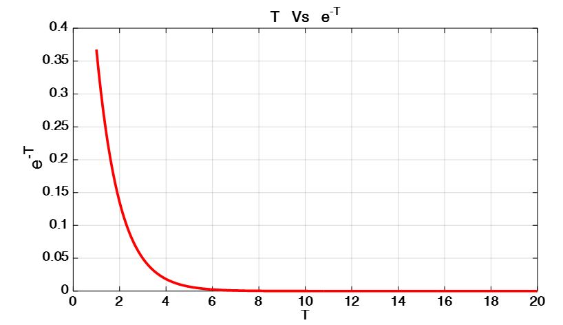
So, if we look at the graph, we can perceive that the function clearly approaches 0 as T→∞. Hence, If Real s>0, the limit in (7) is zero.

Laplace Transform Key Takeaways

The Laplace transform is a powerful mathematical tool with broad applications in engineering, physics, and control systems. It simplifies the analysis of complex continuous-time signals and systems, allowing for the transformation of differential equations into algebraic equations. Understanding the conditions for convergence and the regions of absolute convergence enhances the practical utility of the Laplace transforms, making it crucial for analyzing and solving real-world engineering problems.