The article provides an overview of impedance measurement in AC circuits, focusing on the use of AC bridges to determine both resistive and reactive components. It explains the principle of bridge balance and the calculation of unknown impedance using standard circuit configurations.
The opposition that a circuit offers to the flow of AC is called impedance. By measuring the voltage and current in an AC circuit and utilizing the following equation
$Z={}^{V}/{}_{I}$
We can obtain the magnitude of circuit impedance. However, it is often desirable to separate impedance into resistive and reactive components. One instrument that is used to measure the separate resistive and reactive parts of an impedance is the AC Bridge. The circuit of the general AC Bridge is shown in figure 1.
- You May Also Read: Wheatstone Bridge Working Principle
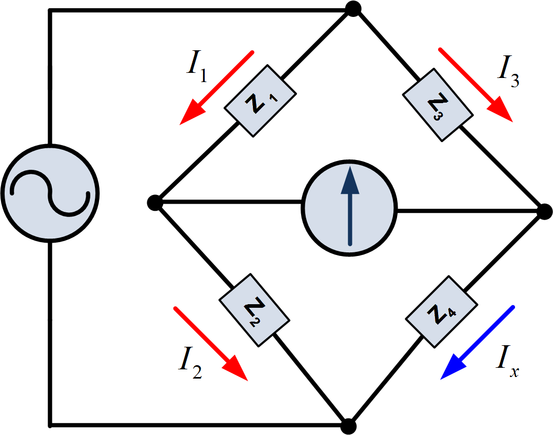
Figure 1: The AC Bridge Circuit
The configuration is similar to that of the Wheatstone bridge, yet distinct differences exist between the components. The AC Bridge has impedance arms, rather than resistance arms; instead of a battery and galvanometer, an AC signal source and null detector are used. If the signal voltage is in the audio range, a set of headphones may be used as the null detector; otherwise, a sensitive AC Voltmeter is used.
As in the Wheatstone bridge, at balance, no current flows through the detector. The voltage from a to c equals that from a to d, so that
${{I}_{1}}{{Z}_{1}}={{I}_{3}}{{Z}_{3}}\text{ (1)}$
Similarly,
${{I}_{2}}{{Z}_{2}}={{I}_{x}}{{Z}_{x}}\text{ (2)}$
It follows that for balanced conditions
\[\frac{{{Z}_{1}}}{{{Z}_{2}}}=\frac{{{Z}_{3}}}{{{Z}_{x}}}\]
\[{{Z}_{x}}={{Z}_{3}}\left( \frac{{{Z}_{2}}}{{{Z}_{1}}} \right)\text{ (3)}\]
In order to obtain balance, at least one of the unknown impedances must have a resistive and reactive components. If Z3 is chosen to be complex, Z1 and Z2 can be conveniently chosen to be purely resistive with a ratio that is a power of 10. Then from equation (3),
${{R}_{x}}+j{{X}_{x}}=({{R}_{3}}+j{{X}_{3}})\left( \frac{{{R}_{2}}}{{{R}_{1}}} \right)\text{ (4)}$
For equation (4) to be satisfied, the real parts of both sides must be equal, and also the imaginary parts of both sides. Equating these parts, we obtain
\[{{R}_{x}}={{R}_{3}}\left( \frac{{{R}_{2}}}{{{R}_{1}}} \right)\text{ (5)}\]
\[{{X}_{x}}={{X}_{3}}\left( \frac{{{R}_{2}}}{{{R}_{1}}} \right)\text{ (6)}\]
A simple inductance bridge is shown in figure 2.

Figure 2: An Inductance Bridge
When the bridge is balanced, we solve for Rx by using equation (5). From equation (6), we then solve for the inductance Lx,
\[\omega {{L}_{x}}=\omega {{L}_{3}}\left( \frac{{{R}_{2}}}{{{R}_{1}}} \right)\text{ }\]
Or
\[{{L}_{x}}={{L}_{3}}\left( \frac{{{R}_{2}}}{{{R}_{1}}} \right)\text{ (7)}\]
Here, from equation (7), we can easily obtain the unknown inductance in the circuit.
- You May Also Read: Maxwell Inductance Bridge Circuit
Impedance Measurement Key Takeaways
Understanding and accurately measuring impedance using AC bridges is crucial for the design, analysis, and maintenance of AC electrical systems. These techniques are widely applied in telecommunications, audio engineering, and circuit diagnostics, where precise separation of resistive and reactive components ensures optimal performance, signal integrity, and system efficiency.