Discrete Time Convolution Properties | Discrete Time Signal

This article provides an overview of discrete-time convolution, including its definition, step-by-step computation process, and key mathematical properties. It also explains how convolution is used to determine the output of linear time-invariant (LTI) systems from known input and impulse responses.

Discrete-Time Convolution

Convolution is such an effective tool that can be utilized to determine a linear time-invariant (LTI) system’s output from an input and the impulse response knowledge.

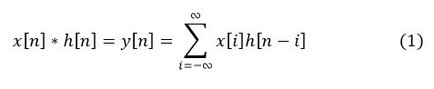
Given two discrete time signals x[n] and h[n], the convolution is defined by

$x\left[ n \right]*h\left[ n \right]=y\left[ n \right]=\sum\limits_{i=-\infty }^{\infty }{{}}x\left[ i \right]h\left[ n-i \right]~~~~~~~~~~~~~~~~~~~~~~~\left( 1 \right)$

The summation on the right side is called the convolution sum.

It should be noted that the convolution sum exists when x[n] and h[n] are both zero for all integers n<0.

If x[n] and  h[n] are zero for all integers n<0, then  x[i]=0 for all integers i<0 and h[n-i] =0 for all integer n-i<0 (or n<i) . Thus the summation on i in (1) may be taken from i=0 to i=n, and the convolution operation is given by,

\[x\left[ n \right]*h\left[ n \right]=\left\{ \begin{matrix} \begin{matrix}\begin{matrix}0, & {} & {}  \\\end{matrix} & n=-1,-2,\ldots   \\\end{matrix}  \\\begin{matrix}\sum\limits_{i=0}^{n}{x\left[ i \right]h\left[ n-i \right]} & {} & {} & n=0,1,2,\ldots   \\\end{matrix}  \\\end{matrix} \right.\text{         (2)}\]

Since the summation in (2) is over a finite range of integers (i=0 to i=n), the convolution sum exists. Hence any two signals that are zero for all integers n<0 can be convolved.

To compute the convolution (1) or (2)   

1. First, change the discrete-time index n to i in the signals x[n] and h[n].
2. Flip the signals h[i] to obtain h[-i] (it is called folding).
3. For each output index n, shift by n to get h[n-i] .(Positive value of n gives right shift.)
4. The product x[n]*h[n] is formed and y[n] is computed by summing the values of x[i]*h[n-i] as i ranges over the set of integers.

Discrete-Time Convolution Example

Suppose that x[n]=aⁿu[n] and h[n]= aⁿu[n] Where u[n] is a discrete-time unit-step function and a and b are fixed non zero  real numbers.

Step 1:

Change discrete time signal index n to i in both signals:

$x\left[ i \right]={{a}^{i}}u\left[ i \right]$

$h\left[ i \right]={{b}^{i}}u\left[ i \right]$

Step 2:

Flip h[i] to get h[-i]:

$h\left[ -i \right]={{b}^{-i}}u\left[ -i \right]$

Step 3:

Shift by n to get h[n-i]:

$h\left[ n-i \right]={{b}^{n-i}}u\left[ n-i \right]$

Step 4:

Find y[n] by summing the product x[i]h[n-i] over a finite range of i:

$y\left[ n \right]=\sum\limits_{i=-\infty }^{\infty }{{}}x\left[ i \right]h\left[ n-i \right]~~~~~~~~~~~\left( 3 \right)$

If x[n] is zero for all integers n<0, then x[i]=0 for all integers i<0, So,

$u\left[ i \right]=\left\{ \begin{matrix}\begin{matrix} 1 & i\ge 0  \\\end{matrix}  \\\begin{matrix} 0 & i<0  \\\end{matrix}  \\\end{matrix} \right.$

Similarly, If h[n] is zero for all integers n<0, then h[n-i]=0 for all integers n-i<0 (or n<i), So,

$u\left[ n-i \right]=\left\{ \begin{matrix}\begin{matrix}1 & i\le n  \\\end{matrix}  \\\begin{matrix}0 & i>n  \\\end{matrix}  \\\end{matrix} \right.$

Thus the summation on i in (3) may be taken from i=0 to i=n and the convolution operation is given by,

$y\left[ n \right]=\sum\limits_{i=0}^{n}{{}}x\left[ i \right]h\left[ n-i \right]$

$y\left[ n \right]=\sum\limits_{i=0}^{n}{{}}{{a}^{i}}{{b}^{n-i}}$

\[y\left[ n \right]={{b}^{n}}\sum\limits_{i=0}^{n}{{}}{{\left( \frac{a}{b} \right)}^{i}}\]

If a=b,

 

$y\left[ n \right]={{b}^{n}}\sum\limits_{i=0}^{n}{{}}{{\left( 1 \right)}^{i}}$

 

If a≠b, then standard math relation gives

 

$\sum\limits_{i=0}^{N-1}{{}}{{\left( r \right)}^{i}}=\frac{1-{{\left( r \right)}^{N}}}{1-r}~~~~~~~~r\ne 1$

Whereas,

 

$y\left[ n \right]=\left\{ \begin{matrix}\begin{matrix}n+1 & ~~~~~~~~~~~~~~~~~a=b  \\\end{matrix}  \\\begin{matrix}\frac{1-{{\left( {}^{a}/{}_{b} \right)}^{n+1}}}{1-\left( {}^{a}/{}_{b} \right)} & a\ne b  \\\end{matrix}  \\\end{matrix} \right.$

Discrete-Time Convolution Properties

The convolution operation satisfies a number of useful properties which are given below:

Commutative Property

If x[n] is a signal and h[n] is an impulse response, then

Associative Property

If x[n] is a signal and h₁[n] and h2[n] are impulse responses, then

Distributive Property

If x[n] is a signal and h₁[n] and h2[n] are impulse responses, then

• You May Also Read: Discrete-Time Graphical Convolution Example

Discrete Time Convolution Properties Key Takeaways

Discrete-time convolution plays a vital role in the analysis and design of digital systems, particularly linear time-invariant (LTI) systems. Understanding how to compute and apply convolution is essential because it provides a systematic method to predict a system’s output based solely on its input signal and impulse response. This capability is especially important in real-world applications such as digital signal processing, communications, image filtering, and control systems, where system behavior must be accurately modeled and manipulated. The properties of convolution—commutativity, associativity, and distributivity—not only simplify computations but also allow for flexible and modular system design.