In linear networks which have inputs that are periodic functions of time, the steady-state currents and voltages produced are periodic, each having identical periods.
Consider an instantaneous power
$\begin{matrix} p=vi & \cdots & (1) \\\end{matrix}$
Where v and i are periodic of period T. that is,
$\begin{align} & v(t+T)=v(t) \\ & and \\ & i(t+T)=i(t) \\\end{align}$
In this case,
$\begin{align} & p(t+T)=v(t+T)i(t+T) \\ & =v(t)i(t) \\ & =\begin{matrix} p(t) & \cdots & (2) \\\end{matrix} \\\end{align}$
Therefore the instantaneous power is also periodic of period T. that is, p repeats itself every T seconds.
The fundamental period T1 of p (the minimum time in which p repeats itself) is not necessarily equal to T, However, but T must contain an integral number of periods T1. In other words,
$\begin{matrix} T=n{{T}_{1}} & \cdots & (3) \\\end{matrix}$
Where n is a positive integer.
As an example, suppose that a resistor R carries a current $i={{I}_{m}}\cos \omega t$ with period $T=\frac{2\pi }{\omega }$ . Then
\[\begin{align} & p=R{{i}^{2}} \\ & =RI_{m}^{2}{{\cos }^{2}}\omega t \\ & =\frac{RI_{m}^{2}}{2}(1+\cos 2\omega t) \\\end{align}\]
Evidently, ${{T}_{1}}=\frac{\pi }{\omega }$ and therefore$T=2{{T}_{1}}$. Thus, for this case, n=2 in (3). This is illustrated by the graph of p and i shown in figure 1 (a).
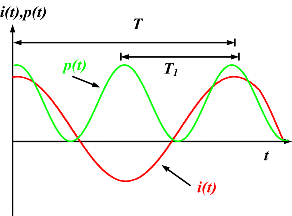
Fig.1 (a): Graph of p and i
If we now take $i={{I}_{m}}\cos (1+\cos \omega t)$ , then
$p=RI_{m}^{2}{{(1+\cos \omega t)}^{2}}$
In this case, ${{T}_{1}}=T=\frac{2\pi }{\omega }$ , and n=1 in (3). This may be seen also from the graph of the function in figure 1 (b).
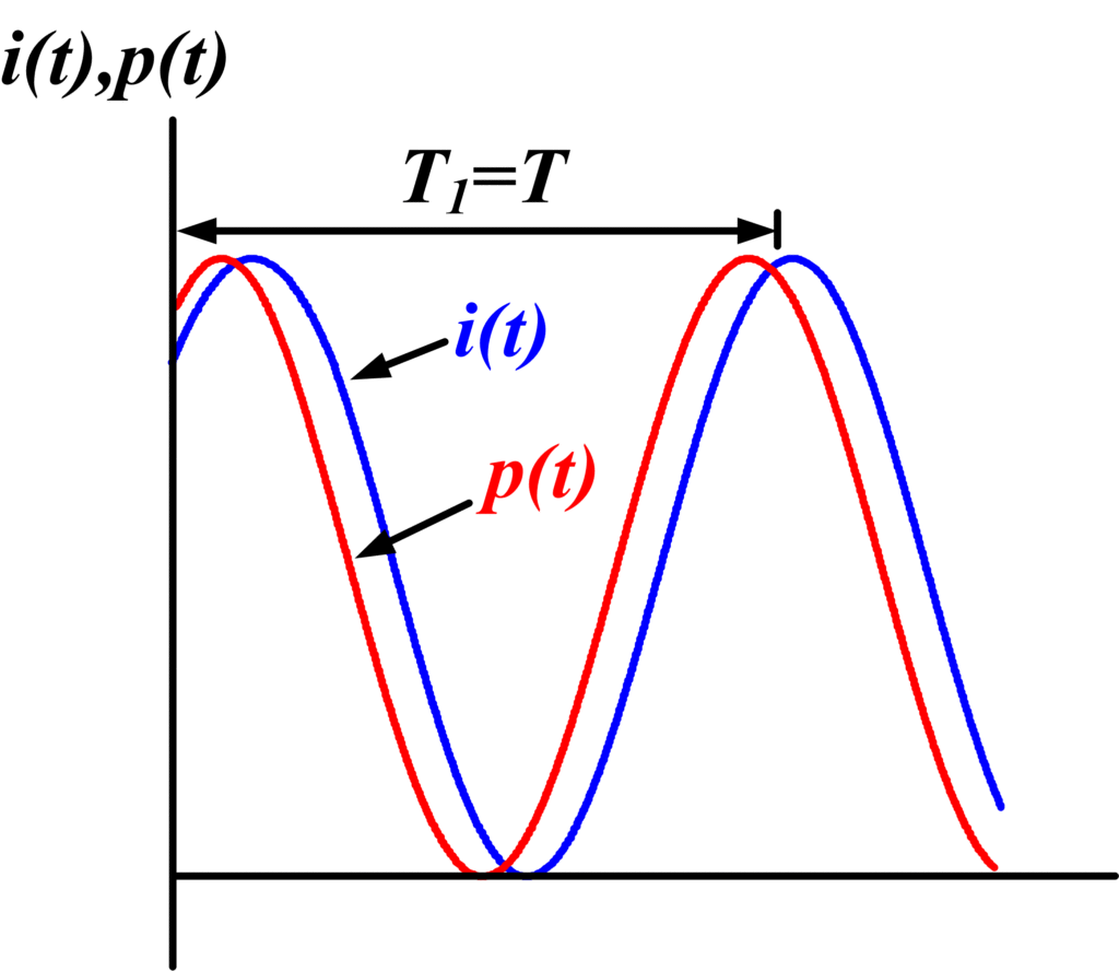
Fig.1 (b): Graph of p and i
Mathematically, the average value of a periodic function is defined as the time integral of the function over a complete period, divided by the period. Therefore, the average power P for a periodic instantaneous power p is given by
$\begin{matrix} P=\frac{1}{{{T}_{1}}}\int_{{{t}_{1}}}^{{{t}_{1}}+{{T}_{1}}}{p\text{ }dt} & \cdots & (4) \\\end{matrix}$
Where t1 is arbitrary.
A periodic instantaneous power p is shown in figure 2.
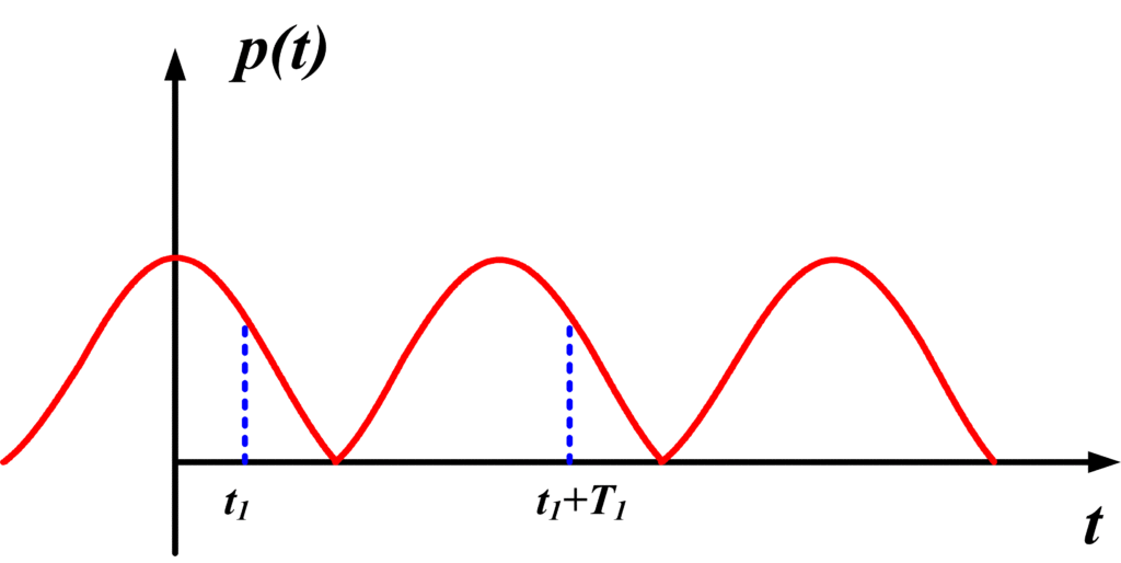
Fig.2: Periodic Instantaneous Power
It is clear that if we integrate over an integral number of periods, say mT1 (where m is a positive integer), then the total area is simply m times that of the integral in (4). Thus we may write
$\begin{matrix} P=\frac{1}{m{{T}_{1}}}\int_{{{t}_{1}}}^{{{t}_{1}}+m{{T}_{1}}}{p\text{ }dt} & \cdots & (5) \\\end{matrix}$
If we select m such that T=mT1 (the period of v and i), then
\[\begin{matrix} P=\frac{1}{T}\int_{{{t}_{1}}}^{{{t}_{1}}+T}{p\text{ }dt} & \cdots & (6) \\\end{matrix}\]
Therefore we may obtain the average power by integrating over the period of v or i.
Let us now consider some examples of the average power associated with sinusoidal currents and voltages. A number of very important integrals which often occur are tabulated in Table 1.
$f(t)$ $\int\limits_{0}^{{}^{2\pi }/{}_{\omega }}{f(t)dt,\text{ }\omega \ne \text{0}}$
$1.\text{ sin(}\omega \text{t+}\alpha \text{),cos(}\omega \text{t+}\alpha \text{)}$ $0$
$2.\text{ sin(n}\omega \text{t+}\alpha \text{),cos(n}\omega \text{t+}\alpha \text{)*}$ $0$
$3.\text{ si}{{\text{n}}^{\text{2}}}\text{(}\omega \text{t+}\alpha \text{),co}{{\text{s}}^{\text{2}}}\text{(}\omega \text{t+}\alpha \text{)}$ ${}^{\pi }/{}_{\omega }$
$4.\text{ sin(m}\omega \text{t+}\alpha \text{)cos(n}\omega \text{t+}\alpha \text{)*}$ $0$
$5.\text{ cos(m}\omega \text{t+}\alpha \text{)cos(n}\omega \text{t+}\beta \text{)*}$ $\left\{ \begin{matrix}
\begin{matrix}
0, & m\ne n \\
\end{matrix} \\
\begin{matrix}
\frac{\pi \cos (\alpha -\beta )}{\omega }, & m=n \\
\end{matrix} \\
\end{matrix} \right.$
* m and n are integers
First, let us consider the general two-terminal device of figure 3, which is assumed to be in AC steady state. If, in the frequency domain,
$Z=\left| Z \right|\angle \theta $
Is the input impedance of the device, then for
\[\begin{matrix} v={{V}_{m}}cos(\omega t+\phi ) & \cdots & (7) \\\end{matrix}\]
We have
\[\begin{matrix} i={{I}_{m}}cos(\omega t+\phi -\theta ) & \cdots & (8) \\\end{matrix}\]

Fig.3: General Two-Terminal Device
Where
\[{{\operatorname{I}}_{m}}=\frac{{{V}_{m}}}{\left| Z \right|}\]
The average power delivered to the device, taking t1=0 in (6), is
$P=\frac{\omega {{V}_{m}}{{I}_{m}}}{2\pi }\int\limits_{0}^{{}^{2\pi }/{}_{\omega }}{\cos (\omega t+\phi )}\cos (\omega t+\phi -\theta )dt$
Referring to table 1, entry 5, we find, for m=n=1, α=ϕ, and β= ϕ-θ,
$\begin{matrix} P=\frac{{{V}_{m}}{{\operatorname{I}}_{m}}}{2}\cos \theta & \cdots & (9) \\\end{matrix}$
Thus the average power absorbed by a two-terminal device is determined by the amplitudes Vm and Im and the angle θ by which the voltage v leads the current i.
In terms of the phasors of v and i,
$V={{V}_{m}}\angle \phi =\left| {{V}_{m}} \right|\angle \phi $
We have, from (9),
\[\begin{matrix} P=\left| V \right|\left| I \right|\cos (ang(V)-ang(I)) & \cdots & (10) \\\end{matrix}\]
Where
$ang(V)=\phi \text{ }and\text{ }ang(I)=\phi -\theta $
Are the angles of the phasors V and I.
If the two-terminal device is a resistor R, then θ=0 and Vm=RIm, so that (9) becomes
${{P}_{R}}=\frac{1}{2}RI_{m}^{2}$
It is worth noting at this point that if i=Im, a constant (DC) current, then ω=ϕ=θ=0, and Im=Idc in (8). In this special case Table 1 does not apply, but by (6) we have
${{P}_{R}}=RI_{dc}^{2}$
In the case of an inductor, θ=90o, and in the case of a capacitor, θ=-90o, and thus for either one, by (9), P=0. Therefore an inductor or a capacitor, or for that matter any network composed entirely of ideal inductors and capacitors, in any combination, dissipates zero average power. For this reason, ideal inductors and capacitors are sometimes called lossless elements. Physically, lossless elements store energy during part of the period and release it during the other part, so that the average delivered power is zero.
A very useful alternative form of (9) may be obtained by recalling that
$Z=\operatorname{Re}(Z)+j\operatorname{Im}(Z)=\left| Z \right|\angle \theta $
And therefore
$Cos\theta =\frac{\operatorname{Re}(Z)}{\left| Z \right|}$
Substituting this value into (9) and noting that Vm=|Z|Im, we have
\[\begin{matrix} P=\frac{1}{2}I_{m}^{2}\operatorname{Re}(Z) & \cdots & (11) \\\end{matrix}\]
Let us now consider this result if the device is a passive load, we know from the definition of passivity that the net energy delivered to a passive load is nonnegative. Since the average power is the average rate at which energy is delivered to a load, it follows that the average power is nonnegative. That is, P≥0. This requires, by (11), that
$\operatorname{Re}\text{ Z(j}\omega \text{)}\ge 0$
Or equivalently
$-\frac{\pi }{2}\le \theta \le \frac{\pi }{2}$
If θ=0, the device is equivalent to a resistance, and if θ=π/2 (or – π/2), the device is equivalent to an inductor (or capacitor). For [stextbox id=”info” caption=”RC Combination “]\[-\frac{\pi }{2}<\theta <0\][/stextbox], the device is equivalent to an RC combination, where for [stextbox id=”info” caption=”RL Combination “]\[0<\theta <\frac{\pi }{2}\][/stextbox], the device is equivalent to an RL combination.
Finally, if |θ|>π/2, then P<0, and the device is active rather than passive. In this case the device is delivering power from its terminals and, of course, acts like a source.
As an example, let us find the power delivered by the source of figure 4.

Fig.4: RL circuit in the AC steady-State
The impedance across the source is
$Z=100+j100=100\sqrt{2}\angle {{45}^{o}}\Omega $
The maximum current is
${{\operatorname{I}}_{m}}=\frac{{{V}_{m}}}{\left| Z \right|}=\frac{1}{\sqrt{2}}A$
Therefore, from (9), the power delivered to Z is
$P=\frac{100}{2\sqrt{2}}\cos {{45}^{o}}=25W$
Alternatively,
$P=\frac{1}{2}{{\left( \frac{1}{\sqrt{2}} \right)}^{2}}100=25W$
We may also note that the power absorbed by the 100 Ω resistor is
${{P}_{R}}=\frac{RI_{m}^{2}}{2}=\frac{(100){{\left( \frac{1}{\sqrt{2}} \right)}^{2}}}{2}=25W$
This power, of course, is equal to that delivered to Z since the inductor absorbs no power.
The power absorbed by the source is
$Pg=-\frac{{{V}_{m}}{{I}_{m}}}{2}\cos \theta =-25W$
Where the minus sign is used because the current is flowing out of the positive terminal of the source. The source, therefore, is delivering 25W to Z. we note that the power flowing from the source is equal to that absorbed by the load, which illustrates the principle of conservation of power.
Average Power Key Takeaways
The concepts of instantaneous and average power in periodic electrical circuits are fundamental in analyzing and designing electrical systems. These power calculations are essential for understanding energy transfer in resistors, inductors, and capacitors, as well as for optimizing circuit performance in AC systems. The use of phasor notation and impedance further enhances the ability to analyze complex circuits efficiently. In practical applications, these principles are crucial for designing power distribution networks, improving energy efficiency, and ensuring the reliability of electrical and electronic systems.