RL Series Circuit Analysis

This article covers RL series circuit analysis both during charging and discharging phases. It explains the current and voltage relationships, the concept of time constant, and the exponential growth and decay of current and voltage in such circuits, along with the corresponding mathematical equations.

When a resistive-inductive (RL) series circuit has its supply voltage switched on, the inductance produces an initial maximum level of counter-emf that gradually falls to zero. The circuit current is zero initially and grows gradually to its maximum level.

The behavior of an RL series circuit is most easily understood by plotting the graphs of instantaneous current versus time and instantaneous inductor voltage versus time. Care must be taken in open-circuiting an RL circuit to avoid an excessively high induce voltage.

At time t=0, the switch in the above circuit is closed. At the instance of switch closure (t=0), a current i tends to flow. However, characteristic of an inductor is to oppose any instantaneous change of current. This property stems from the relationship of the inductor voltage;

${{V}_{L}}=L\frac{di}{dt}$

From this expression, the voltage across an inductor depends on the rate of change of current. In other words, it is the property of the inductor to keep the value of current same as it was before the switch was closed. Prior to closure, i=0. Therefore current must be zero at t=0. Only after the switch has been closed for a sufficiently long period of time is the current able to build up to a steady state value.

Let’s apply Kirchhoff’s voltage law to above RL series circuit.

\[\begin{matrix}   E={{E}_{R}}+{{E}_{L}} & {} & \left( a \right)  \\\end{matrix}\]      

From Ohm’s law;

${{V}_{R}}=iR$

And inductor voltage

${{V}_{L}}=L\frac{di}{dt}$

So, the equation (a) would be;

$E=iR+L\frac{di}{dt}$

Dividing both sides by “R”

$\frac{E}{R}=i+\frac{L}{R}\frac{di}{dt}$

$\frac{E}{R}-i=\frac{L}{R}\frac{di}{dt}$

                 $\frac{di}{\frac{E}{R}-i}=\frac{R}{L}dt$            

Integrating both sides;

\[\begin{matrix}   \int{\frac{di}{\frac{E}{R}-i}}=\int{\frac{R}{L}dt} & {} & \left( b \right)  \\\end{matrix}\]                  

Let’s assume

$u=\frac{E}{R}-i$

Differentiating both sides,

$du=-di$

Putting values back in eq. (b) yields

$\underset{{{u}_{i}}}{\overset{{{u}_{f}}}{\mathop \int }}\,\frac{du}{u}dt=\underset{{{t}_{0}}}{\overset{{{t}_{f}}}{\mathop \int }}\,\frac{R}{L}dt$

Whereas u_i and u_f are initial and final values. After integrating, we have

$\ln \left| u \right|=-\frac{R}{L}\left( t \right)$

$\ln \left( {{u}_{f}} \right)-\ln \left( {{u}_{i}} \right)=-\frac{R}{L}\left( {{t}_{f}}-{{t}_{0}} \right)$

${{t}_{0}}=0$

$\ln \frac{{{u}_{f}}}{{{u}_{i}}}=-\frac{R}{L}{{t}_{f}}$

Taking exponent on both sides, we have

$\frac{{{u}_{f}}}{{{u}_{i}}}={{e}^{-\text{ }\frac{R}{L}{{t}_{f}}}}$

Now

${{u}_{f}}={{u}_{i}}{{e}^{-\text{ }\frac{R}{L}{{t}_{f}}}}$

As we know that:

${{u}_{f}}=\frac{E}{R}-{{i}_{f}}$

${{u}_{i}}=\frac{E}{R}-{{i}_{i}}$

Then,

$\frac{E}{R}-{{i}_{f}}=\left( \frac{E}{R}-{{i}_{i}} \right){{e}^{-\text{ }\frac{R}{L}{{t}_{f}}}}$

And

$~{{i}_{i}}=0$                      (Initially, when S=0)

So,

$\frac{E}{R}-{{i}_{f}}=\frac{E}{R}{{e}^{-\text{ }\frac{R}{L}{{t}_{f}}}}$

So the final expression of current would be,

$i=\frac{E}{R}\left( 1-{{e}^{-\text{ }\frac{R}{L}t}} \right)\text{     }\cdots \text{   (c)}$

While

 ${{i}_{max}}=\frac{E}{R}$

A plot of equation (c) is an exponential curve as shown in fig.

• You May Also Read: RC Circuit Analysis

The typical growth of current with time for a series RL Circuit from the instant of supply voltage switch-on.

After the switch is closed, the current in the circuit rises initially, then levels off and approaches the final steady-state value.

From equation (c), we can extract inductor voltage expression as well;

$i=\frac{E}{R}-\frac{E}{R}{{e}^{-\text{ }\frac{R}{L}t}}$

Differentiating both sides,

$\frac{di}{dt}=\frac{E}{L}{{e}^{-\text{ }\frac{R}{L}t}}$

$L\frac{di}{dt}=E{{e}^{-\text{ }\frac{R}{L}t}}$

Since

${{V}_{L}}=L\frac{di}{dt}$

So,

\[\begin{matrix}   {{V}_{L}}=E{{e}^{-\frac{R}{L}t}} & {} & \left( d \right)  \\\end{matrix}\]     

Equation (d) describes the decaying behavior of inductor voltage V_L as shown in the figure.

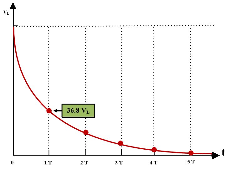
Graph if inductor voltage V_L versus time t for a series RL Circuit. The voltage falls by 63.2% of its maximum value at t=L/R and by 99.3% of its maximum at t=5 L/R.

Time Constant

After the switch of the above RL circuit is closed, we have seen that the current rises exponentially. The rate of rising depends on the exponent -t/𝝉. In term of circuit quantities;

$\frac{t}{\tau }=\frac{t}{{}^{L}/{}_{R}}$

The denominator (L/R) of this expression has a special significance in circuit analysis. It is called the time constant of an RL series circuit and is represented by Greek letter ().

$\tau ={}^{L}/{}_{R}$

Whenever the time constant 𝝉 equals the time, t, then t/𝝉 =1. Under this condition, refer to the following figure, the current has

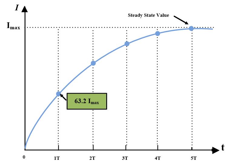
Graph of current i versus time t for a series RL Circuit. The current increases to 63.2% of its maximum level at t=L/R and to 99.3% of its maximum at t=5 L/R.

risen to 63.2 percent of its final value. Thus, the time constant for RL circuit may be defined as the:

The time it takes the instantaneous current to reach 63.2 percent of its final value.

As mentioned earlier current rises exponentially but never reaches the final value until t=∞. We must, therefore, consider some time after which, a constant current flows. When the current has risen to 98 % of its final value, we may say the current is constant. The current reaches 98 % of its final value in five-time constants. Thus,

$5\tau =5\frac{L}{R}$

For this reason, it is not necessary to have the universal exponential curve extend farther than 5-time constants.

RL Series Circuit Discharging

We analyzed an RL circuit when a dc voltage was applied. We now analyze what happens in a circuit containing an inductor when the switch is opened. Consider the following circuit:

We have stated that a characteristic of an inductor is that the current through it cannot change instantaneously. In other words, an inductor opposes any change of current. Since the voltage source was connected when the switch was closed, a current had to flow. Now we begin by applying Kirchhoff’s voltage law to the above circuit.

${{V}_{R}}+{{V}_{L}}=0$

$iR+L\frac{di}{dt}=0$

$i+\frac{L}{R}\frac{di}{dt}=0$

$\frac{L}{R}\frac{di}{dt}=-i$

$\frac{di}{i}=\frac{R}{L}dt$

Integrating both sides

$\underset{{{i}_{i}}}{\overset{{{i}_{f}}}{\mathop \int }}\,\frac{di}{i}=-\underset{{{t}_{0}}}{\overset{{{t}_{f}}}{\mathop \int }}\,\frac{R}{L}dt$

$\ln |\frac{{{i}_{f}}}{{{i}_{i}}}|=-\frac{R}{L}\left( {{t}_{f}}-{{t}_{i}} \right)$

As we know that

${{t}_{0}}=0$                                                   (Initially)

Taking exponents on both sides;

${{i}_{f}}={{i}_{i}}{{e}^{-\frac{R}{L}{{t}_{f}}}}$

i_f and i_i are final and initial values of current.

${{i}_{i}}=\frac{E}{R}$

Whereas E/R is the maximum value of the current and E is the Source voltage.

So, the final expression for the current would be;

\[\begin{matrix}   i=\frac{E}{R}{{e}^{-\frac{R}{L}t}} & {} & \left( e \right)  \\\end{matrix}\]          

Where L is the value of an inductor in Henry and R is the value of resistance.

When the time constant, 𝝉, equals the time, t, then t/𝝉=1. Under this condition, current decays by 63 percent of its initial value. Almost all the electrical energy stored in the inductor at t=0 is converted to heat after 5𝝉.    

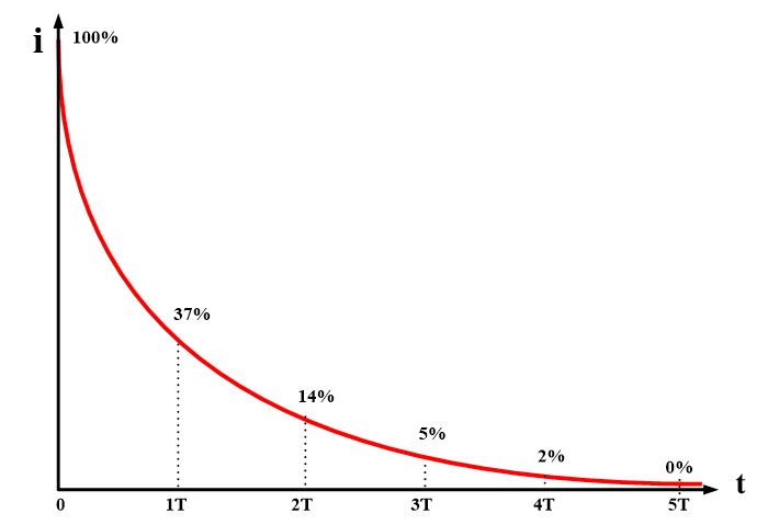
When the voltage is switched off, I decreases exponentially from the maximum level.

From equation (e) we can obtain an expression for inductor voltage for discharging circuit. Taking derivative on both sides of equation (e)

$\frac{di}{dt}=\frac{E}{R}{{e}^{-\frac{R}{L}t}}\left( -{}^{R}/{}_{L} \right)$

$L\frac{di}{dt}=-E{{e}^{-\frac{R}{L}t}}$

So final expression for inductor voltage would be;

^{${{V}_{L}}=-E{{e}^{-\frac{R}{L}t}}$}

You May Also Read: RL Circuit Analysis using Matlab

RL Series Circuit Analysis Key Takeaways

Understanding RL series circuit analysis, including both the charging and discharging phases, is crucial for numerous practical applications in electrical engineering. The concepts of current-voltage relationships, time constant, and exponential behavior play a significant role in the design and operation of various electrical systems. For example, RL circuits are foundational in power supply systems, where inductance and resistance determine how current builds up or decays, influencing circuit performance. The time constant, which determines how quickly the current stabilizes, is especially important in devices like filters, where controlling the rate of current change is essential. In power management, the ability to predict the exponential rise and decay of current allows engineers to design circuits that avoid electrical surges or unwanted oscillations, ensuring system stability. Furthermore, RL circuits are used in inductive loads, signal processing, and energy storage applications, where the management of current flow and voltage is essential for efficiency and safety.