The article provides an overview of frequency response in electrical circuits, explaining how circuit behavior changes with frequency variations, particularly in RLC circuits. It discusses key concepts such as attenuation, frequency response curves, cutoff frequency, filter types (low-pass, high-pass, bandpass, and notch filters), bandwidth, center frequency, and filter quality (Q factor), with supporting examples and formulas.
The reaction of a circuit has to change in frequency is referred to as its Frequency Response. For example, consider the parallel RLC circuit shown in Figure 1. If the operating frequency of the circuit increases, Here’s what happens:
• The reactance of the inductor increases because of XL=2πfL. The increase in XL causes the inductor current (IL) to decrease.
• The reactance of the capacitor decreases, because of XC =1/2πfC. The decrease in XC causes the capacitor current (IC) to increase.
• The changes in IL and IC cause the total circuit current to change, as well as the circuit phase angle is (θ)
These changes are collectively referred to as the circuit frequency response.
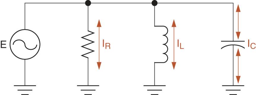
Figure 1: Parallel RLC Circuit Diagram
The subject of frequency response is complex, with many principles and concepts. In this section, we will introduce the most general principles.
Attenuation
Every circuit responds to a change in operating frequency to some extent. The changes may be too subtle to observe, or they may be dramatic. An example of the latter is illustrated in Figure 2.
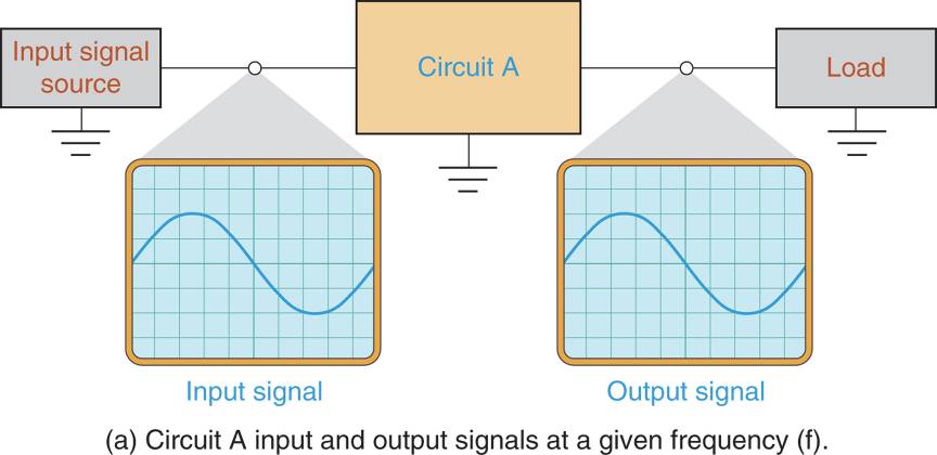
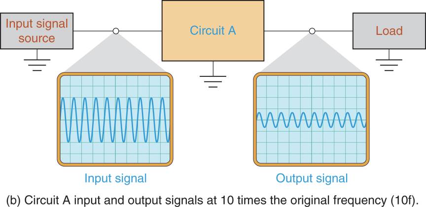
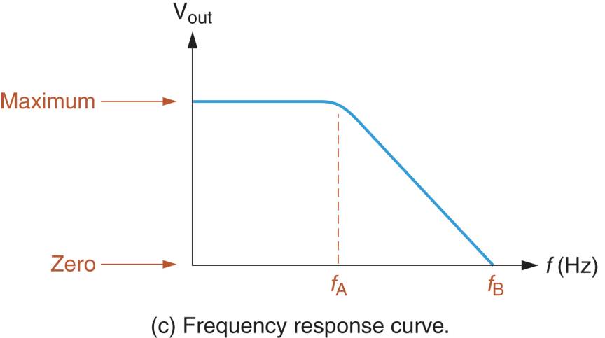
Figure 2: Attenuation
The circuit represented in Figure 2a has input and output waveforms that are nearly identical. When the input frequency is increased by a factor of ten (as shown in Figure 2b), the amplitude of the circuit output drops significantly. Any signal loss caused by the frequency response of a circuit is referred to as Attenuation.
The frequency response just described can be graphed as shown in Figure 2c. As you can see, the amplitude of the circuit output stays relatively constant over the range of frequencies below the frequency labeled fA.
As operating frequency increases abut fA, the attenuation introduced by the circuit causes the amplitude to drop. If the operating frequency reaches the frequency labeled fB, the output amplitude decreases to zero. (This means the circuit has no output signal, even though it still has an input signal)
Frequency Response Curves
The frequency response of a circuit is commonly described in terms of the effect that a change in operating frequency has on the ratio of output amplitude to input amplitude. For example, the curve in Figure 3 represents the frequency response of a circuit with a maximum value of \[\frac{{{V}_{out}}}{{{V}_{in}}}=1\].
According to the curve, the ratio of Vout and Vin decreases from:
\[\begin{matrix}\frac{{{V}_{out}}}{{{V}_{in}}}=1 & {} & at\text{ }{{f}_{A}} \\\end{matrix}\]
to
\[\begin{matrix}\frac{{{V}_{out}}}{{{V}_{in}}}=0 & {} & at\text{ }{{f}_{B}} \\\end{matrix}\]
The ratio of the circuit’s output amplitude to its input amplitude is referred to as Gain. As such, the circuit represented by the curve in Figure 3 is described as having a maximum Voltage Gain of one (1). A gain of one is commonly called Unity Gain.
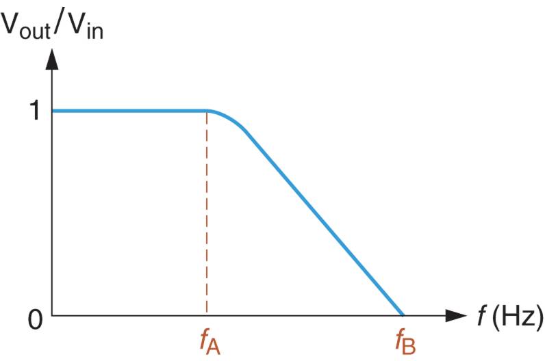
Figure 3: A Graph of Voltage Gain vs Frequency
Cutoff Frequency (fc)
A frequency response curve is a graph that shows the effect that frequency has no gain. In most cases, these curves use a power ratio as the indicator of gain. For example, the curve gain in Figure 4 represents the relationship between frequency and Power gain (the ratio of output power to input power)
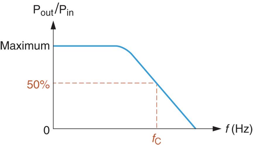
Figure 4: A Graph of Power Gain vs Frequency
The frequency at which the power gain of a circuit drops to 50% of its maximum value is referred to as its Cutoff frequency (fr). The cutoff frequency is identified on the curve in Figure 4.
By convention, the cutoff frequency on a curve is the dividing line between acceptable and unacceptable output levels from a component or circuit. When the power gain of a circuit is below 50% of its maximum value, the output has been attenuated to the point of being considered unacceptable.
It should be noted that the 50% standard for cutoff frequency is an arbitrary value; that is, it is used only because it is agreed upon by professionals in the field. The cutoff frequency of a component or circuit is determined by its resistive values.
Filters
Many circuits are designed for specific frequency response characteristics, that is, they are designed to pass a specific range of frequencies from input to output while blocking (or rejecting) others. These circuits are generally referred to as Filters.
There are four characteristic filter response curves. These curves are shown in Figure 5.
Figure 5a shows the response curve for a low pass filter. A low pass filter is designed to pass all frequencies below its cutoff frequency (fC). For example, a low pass filter with a value of fC = 1000Hz will pass all frequencies below 1000Hz.
In contrast, a high pass filter is designed to pass all frequencies above its cutoff frequency (as shown in Figure 5b).
A Bandpass Filter is one is designed to pass the band of frequencies that lies between two cutoff frequencies, labeled fC1 and fC2, as shown in Figure 5c.
In contrast, a band stop filter, or notch filter, is designed to block the band of frequencies that lies between its cutoff frequencies. As shown in Figure 5d, the notch filter passes frequencies that are below fC1 and above fC2.
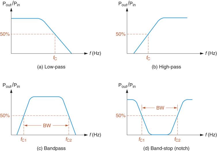
Figure 5: Filter Frequency Response Curves
Because bandpass and notch filters have two cutoff frequencies, two values are used to describe their operation that are not commonly applied to low pass and high pass filters. These values are called bandwidth and center frequency.
Bandwidth and Center Frequency
The range (or band) of frequencies between the cutoff frequencies of a filter is referred to as its Bandwidth. The concept of bandwidth is illustrated in Figure 6.
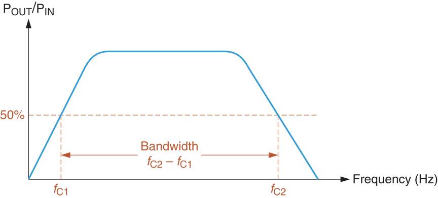
Figure 6: Bandwidth
As shown in the figure, bandwidth is equal to the difference between the cutoff frequencies. By Formula
\[\begin{matrix}BW={{f}_{C2}}-{{f}_{C1}} & {} & \left( 1 \right) \\\end{matrix}\]
Where
BW= the bandwidth of the component or circuit, in Hz
fC2= the upper cutoff frequency
fC1= the lower cutoff frequency
The bandwidth of a filter can be calculated as demonstrated in example 1.
Example 1
A bandpass filter has the frequency response shown in figure 6a. Calculate the circuit bandwidth.
Solution
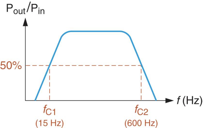
Figure 6a. Frequency Response of a Bandpass Filter
Using the cutoff frequencies shown on the curve, the filter bandwidth is found as:
$BW={{f}_{C2}}-{{f}_{C1}}=600Hz-15Hz=585Hz$
This result indicates that there is a 585 Hz spread between the cutoff frequencies of the circuit.
Center Frequency (f0)
To accurately describe the frequency response of a bandpass or notch filter we need to know more than its bandwidth. We also need to know where the frequency response curve is located on the frequency spectrum.
For example, consider the bandpass curves shown in Figure 7. Each curve has a bandwidth of 100Hz, yet they have different cutoff frequencies and therefore are not the same curve. To distinguish between them, we must identify the center frequency of each curve.
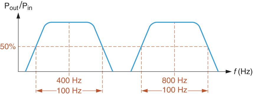
Figure 7: Center Frequency and Bandwidth
Technically defined, the center frequency is the frequency that equals the geometric average of the cutoff frequencies. The geometric average of any two values equals the square root to their product. Therefore, the center frequency is found as:
$\begin{matrix}{{f}_{0}}=\sqrt{{{f}_{C1}}{{f}_{C2}}} & {} & \left( 2 \right) \\\end{matrix}$
Example 2 shows how the center frequency is calculated for a filter.
Example 2
A bandpass filter has the following values:
$\begin{align}& {{f}_{C1}}=50Hz \\& {{f}_{C2}}=400Hz \\\end{align}$
Calculate the value of the circuit’s center frequency.
Solution
Using the values given, the value of f0 is found as:
${{f}_{0}}=\sqrt{{{f}_{C1}}\times {{f}_{C2}}}=\sqrt{\left( 50Hz \right)\times \left( 400Hz \right)}=141Hz$
When we first hear the term center frequency, we tend to picture a frequency that is halfway between the cutoff frequencies. However, this is not always the case. Consider the result in example 2. Obviously, 141 Hz is not halfway between 50Hz and 400Hz. However, it is at the geometric center of the two values meaning that the ratio of fo to fC1 equals the ratio of fC2 to fo. By Formula,
\[\begin{matrix}\frac{{{f}_{0}}}{{{f}_{C1}}}=\frac{{{f}_{C2}}}{{{f}_{0}}} & {} & \left( 3 \right) \\\end{matrix}\]
If we apply this relationship to the values obtained in the example, we get:
\[\frac{141.4Hz}{50Hz}=\frac{400Hz}{141.4Hz}\]
which is true. When you solve the ratios with your calculator, you see that they are equal. This is always the case for the geometric average of two values.
Filter Quality (Q)
The quality (Q) of a bandpass or notch filter is the ratio of its center frequency to its bandwidth by the formula:
\[\begin{matrix}Q=\frac{{{f}_{0}}}{BW} & {} & \left( 4 \right) \\\end{matrix}\]
Example 3 illustrates how to compute the filter quality (Q) for a bandpass filter.
Example 3
Determine the Q of the bandpass filter represented by the curve in figure 7a.
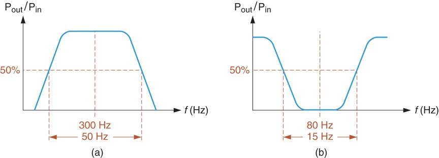
Figure 7a
Solution
The curve has values for f0=300 Hz and BW=50Hz. Using these two values, the Q of the filter is
\[Q=\frac{{{f}_{0}}}{BW}=\frac{300Hz}{50Hz}=6\]
Note that the result has no unit of measure since it is a ratio of one frequency to another.
There is an important point to be made at this time. Equation 4 is somewhat misleading because it implies that the value of Q depends on the values of center frequency and bandwidth.
However, this is not the case. The Q of a filter and its center frequency are both determined by circuit component values. Once their values are known, the filter Q and center frequency are used to calculate the bandwidth of the circuit, as follows:
\[\begin{matrix}BW=\frac{{{f}_{0}}}{Q} & {} & \left( 5 \right) \\\end{matrix}\]
Example 4 provides a more practical application of the relationship among Q, center frequency, and bandwidth.
Example 4
Through a series of calculations, a bandpass filter is determined to have values of Q=4.8 and f0=960 Hz. Calculate the circuit bandwidth.
Solution
Using the calculated values of Q and center frequency, the circuit bandwidth is found as:
\[BW=\frac{{{f}_{0}}}{Q}=\frac{960Hz}{4.8}=200Hz\]
The methods used to calculate the values of Q and fo vary from one type of filter to another. For now, we simply want to establish the fact that filter bandwidth is determined by the circuit values of Q and fo.
Average Frequency (fAVE)
Every bandpass and notch filter has both a center frequency and an average frequency. This average frequency is the frequency that lies halfway between the cutoff frequencies. By Formula,
\[\begin{matrix}{{f}_{AVE}}=\frac{{{f}_{C1}}+{{f}_{C2}}}{2} & {} & \left( 6 \right) \\\end{matrix}\]
As demonstrated in example 5, there can be a significant difference between the values of f0 and fAVE.
Example 5
Determine the values of f0 and fAVE for the circuit represented by the curve in figure 7b.
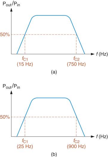
Figure 7b
Solution
Using the values shown on the curve, the geometric average of the cutoff frequencies (f0) is found as:
${{f}_{0}}=\sqrt{{{f}_{C1}}\times {{f}_{C2}}}=\sqrt{\left( 15Hz \right)\times \left( 750Hz \right)}=106Hz$
The algebraic average of the cutoff frequencies is found as:
\[{{f}_{AVE}}=\frac{{{f}_{C1}}+{{f}_{C2}}}{2}=\frac{15Hz+750Hz}{2}=382.5Hz\]
Frequency Scales
Up to this point, we have shown only the given and calculated frequencies on our response curves. In practice, frequency response curves are commonly plotted using frequency scales like those shown in Figure 8.
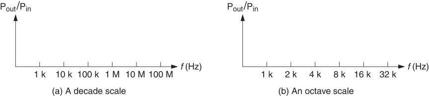
Figure 8: logarithmic frequency scales
The scales shown in the figure are referred to as Logarithmic Scales, meaning that the frequency spread from one increment to the next increases at a geometric rate. In a geometric scale, the value of each increment is a whole number multiple of the previous increment. For example, the value of each increment in Figure 8a is ten times the value of the previous increment.
A frequency multiplier of 10 is referred to as a Decade. For this reason, the scale shown in Figure 8a is called a Decade Scale. In contrast two (2) is the multiplier used from one increment to the next in Figure 8b. A frequency multiplier of 2 is referred to as an Octave, so the scale is called an Octave scale.
Note that both decade and octave scales are used in practice. When a large frequency range is needed, a decade scale is used. When a more precise representation over a smaller frequency range is needed, an octave scale may be used.
When a logarithmic scale is used, the center frequency (which is the geometric average of the cutoff frequencies) falls in the physical center of the curve. This point is illustrated in Figure 9. The curve shown was plotted using assumed cutoff frequencies of 8Hz and 128Hz. Using equation 2, the center frequency of the curve can be found as:
${{f}_{0}}=\sqrt{{{f}_{C1}}\times {{f}_{C2}}}=\sqrt{\left( 8Hz \right)\times \left( 128Hz \right)}=32Hz$
As shown in Figure 9a, the geometric center frequency falls very close to the physical center of the curve. If an algebraic scale were used, f0 would fall very close to the left end of the scale as shown in Figure 9b.
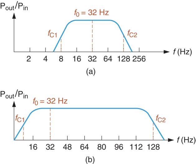
Figure 9: plots for f0 and fAVE
Critical Frequencies: Putting IT Altogether
Low pass and high pass filters are identified using a single cutoff frequency, as shown in Figure 5. Low pass filters have an upper cutoff frequency (fC1). In either case, the cutoff frequency is the operating frequency where the ratio of output power to input power equals 50% of its maximum value. The value of the cutoff frequency for either response curve depends on component values in the circuit itself.
Bandpass and band stop (or notch) filters each have two cutoff frequencies as shown in Figure 5. A bandpass filter passes the band of frequencies that lie between its cutoff frequencies. A notch filter blocks (attenuates) the band of frequencies that lies between its cutoff frequencies.
Bandpass and notch filters are normally described in terms of their center frequency and bandwidth (BW). The center frequency equals the geometric average of cutoff frequencies, and the bandwidth equals the difference between them. In effect, the center frequency tells us where the curve is located on the frequency spectrum, while the bandwidth tells us the range of frequencies that are passed (or blocked) by the filter.
The average frequency of a bandpass or notch filter equals the algebraic average of its cutoff frequencies. The value of fAVE of a bandpass or notch filter equals the algebraic average of its cutoff frequencies. The value of fAVE (not shown in the figure) falls halfway between the cutoff frequencies.
Most frequency response curves are plotted on logarithmic scales. The frequency spread from one increment to the next on a logarithmic scale increases at a geometric rate. That is, the value of each increment is a whole number multiple of the previous increment.
The two most commonly used logarithmic scales are the decade and octave scales. A decade scale is constructed so that the value of each increment is ten times the value of the previous increment. An octave scale uses two as the multiplier between increments.
Frequency Response Key Takeaways
Frequency response is a crucial concept in electrical circuits, particularly in applications involving signal processing, communication systems, and electronic filters. Understanding how circuits react to different frequencies allows engineers to design systems that effectively manage signal attenuation, amplify desired signals, and filter out unwanted noise. Filters such as low-pass, high-pass, bandpass, and notch filters play vital roles in audio processing, radio transmission, medical devices, and control systems. The concepts of bandwidth, center frequency, and quality factor (Q) ensure precise tuning of circuits for optimal performance.