When a series RL circuit is connected across a supply, voltage and current transients occur until the current attains a steady-state condition. Consider the circuit figure 1, where R represents the coil’s resistance or an external resistance. When the switched is closed, current begins to flow into the inductance. The rate of change of current, roc i, will be greatest when the switched is closed. Current and voltage transients will be produced until the current reaches a steady-state level of E/R, at which time the coil effect will be negligible.
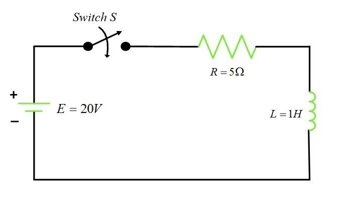
Fig.1: Circuit to illustrate RL Time Constant
The time required for the transient current to reach 63.2 % of its maximum value can be calculated by the following equation:
\[\tau =\frac{L}{R}\]
Where
τ= time constant in seconds
L= inductance in Henry
R=resistance in ohms
The time constant τ also represents the time required for the steady-state current to drop 63.2 % when the inductive circuit is opened.
- You May Also Read: RL Circuit Time Constant using Matlab
Example
Determine the time constant of the RL Circuit in figure 1 when the switch is closed.
Solution
\[\tau =\frac{L}{R}=\frac{1}{5}=0.2s\]
Universal Time Constant Curve
Because of the identical nature of the transient response in RL and RC circuits, a common graph may represent both, as in figure 2.
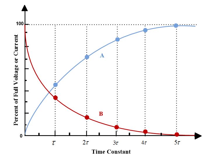
Fig.2: Universal Time Constant Curves for RC and RL Circuits
The X-axis represents time constants, and the Y-axis represents a percentage of full current or voltage. For RL circuits, curves A and B represents iL and VL respectively. For RC circuits, curves A and B represents VC and iC respectively. For both cases, the rise or fall of the curve changes by 63 % in one time constant.
With information obtained from the graph, it is possible to determine the voltage across a capacitor and its charge at any time constant, or fraction thereof, during the charging or discharging cycle. The same statement applies to the inductive circuit.
Exponential Nature of Time Constant Curve
The universal time constant graph is based on the following equation, which gives the exponential rise in a capacitive circuit and is derived from the calculus:
\[{{v}_{C}}=E(1-{{e}^{-\frac{t}{RC}}})\]
Where
E=supply voltage
-t/RC=ratio of time to RC time constant
Note: the value of –t/RC is the ratio of actual time of t to the RC time constant.
The following example illustrates the use of this above-mentioned equation when the time elapsed t is jut equal to one time constant. In other words, when t=RC=τ.
Example
Determine the rise of voltage across a capacitor in a series RC Circuit in one time constant.
Solution
For 1τ, -t/RC=-1. Therefore:
\[{{v}_{C}}=E(1-{{e}^{-\frac{t}{RC}}})=E(1-{{e}^{-1}})=0.6321E\]
The voltage across the capacitor will rise to 0.6321, or 63.21 % of the supply voltage in RC seconds, the value of 1 on the time constant curve. By plotting VC for different time constants, we obtain the universal curve A of figure 2.
The charging current in a series RC Circuit can be calculated for any time constant with the following formula:
\[i={{\operatorname{I}}_{max}}{{e}^{-\frac{t}{RC}}}\]
This equation is the decreasing form of the exponential curve (curve B in figure 2).
Example
Calculate the value of capacitive current in a series RC Circuit in one time constant.
Solution
For 1τ, -t/RC=-1. Therefore:
\[i\text{=}{{I}_{\max }}{{e}^{-\frac{t}{RC}}}={{I}_{\max }}{{e}^{-1}}\text{=0}\text{.367}{{\text{I}}_{\text{max}}}\]
The charging current in an RC circuit will have dropped to 0.3679, or 36.8 % of its maximum E/R value in one time constant after charging begins. If different time constants plotted, curve B of figure 2 results.
For the series RL circuit, the following formula is used to calculate the inductive current at any instant:
\[i=\operatorname{I}(1-{{e}^{-\frac{tR}{L}}})\]
Example
Refer to figure 3, calculate iL at a time 0.2 ms after the circuit is closed.
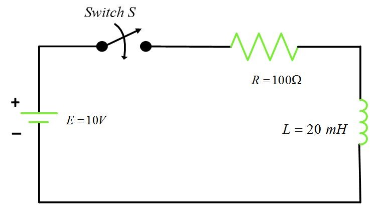
Fig.3: Series RL Circuit for the above example
Solution
First, find tR/L:
\[\frac{tR}{L}=\frac{0.2*{{10}^{-3}}*100}{20*{{10}^{-3}}}=-1\]
Now, calculate iL:
\[i=\frac{10}{100}(1-{{e}^{-1}})=0.0632A\]
This value represents the current in the circuit after one time constant.
The percentages of the steady state values reached after the passage of some of the commonly used multiples of the time constants are tabulated in table 1. For example, for τ=0.5, the percentage is 40 %.
| TIME CONSTANT ( τ ) | % ULTIMATE VALUE |
|---|---|
| 0.1 | 10 |
| 0.5 | 40 |
| 0.7 | 50 |
| 0.9 | 60 |
| 1 | 63.2 |
| 2 | 86.5 |
| 3 | 95.1 |
| 4 | 98.2 |
| 5 | 99.3 |
- You May Also Read: RC Circuit Time Constant
RL Circuit Time Constant Key Takeaways
Understanding the RL circuit time constant and its exponential behavior is crucial for designing and analyzing electrical circuits, particularly in power systems, signal processing, and control applications. These principles help engineers predict transient responses, optimize circuit performance, and ensure efficient energy storage and dissipation. Whether in motor control, filter design, or timing circuits, mastering time constant calculations enhances the reliability and functionality of modern electrical and electronic systems.