The article discusses the Root Locus method, a graphical technique used in control systems to analyze system stability as a gain parameter varies, and outlines the standard rules for constructing root locus plots. It also demonstrates how to implement root locus analysis using MATLAB with example code and visualization.
what is Root Locus
[stextbox id=’info’ caption=’Root Locus’]Root Locus method is a widely used graphical technique to analyze how the system roots vary with variation in particular parametric quantity, generally a gain in a feedback control system. Root Locus is a process practiced as a stability measure in classical control which can find out system stability by plotting closed loop transfer function poles as a function of a gain parameter in the complex s-plane.[/stextbox]
Consider as a standard form for root locus construction, the open-loop transfer function given by;
\[GH(s)=K\frac{(s+{{z}_{1}})(s+{{z}_{2}})\cdots (s+{{z}_{z}})}{(s+{{p}_{1}})(s+{{p}_{2}})\cdots (s+{{p}_{p}})}\]
Where there are z finite zeros and p finite poles of GH(s). We write the characteristic equation for the system given below;
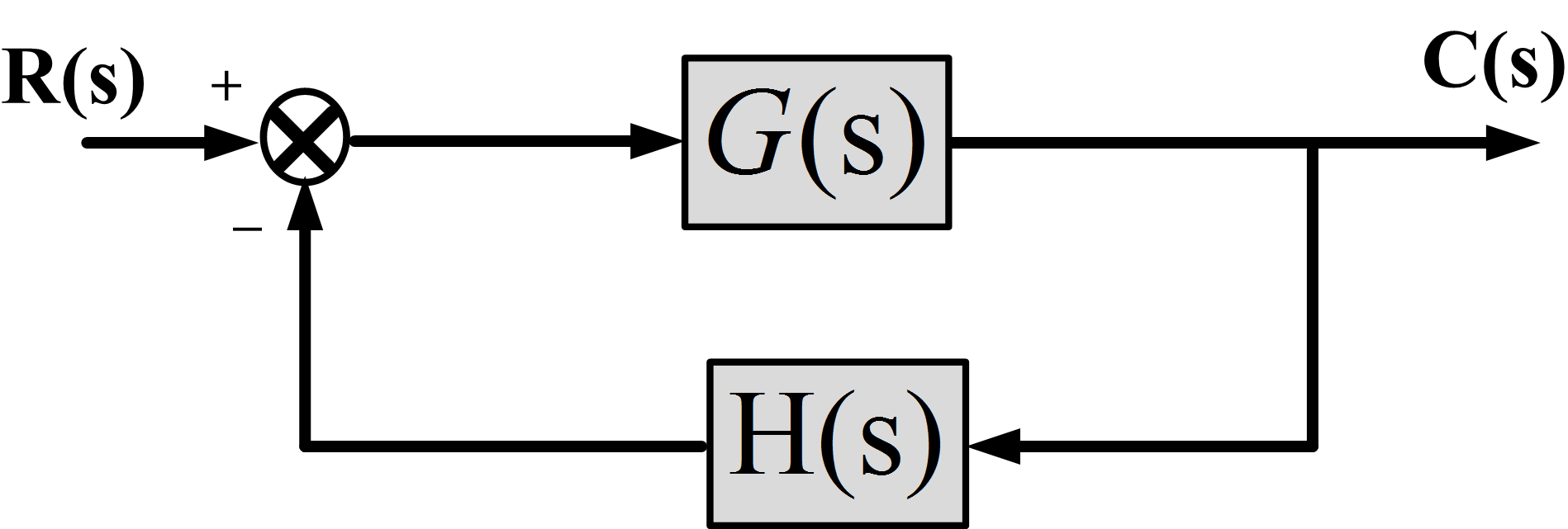
Figure 1: Closed-Loop System
\[\frac{C(s)}{R(s)}=\frac{G(s)}{1+G(s)H(s)}\]
The characteristic equation of this closed loop system would be
$1+G(s)H(s)=0$
Or
$G(s)H(s)=-1$
The closed loop poles are the values of s that satisfy both of the following conditions:
Angle Condition:
$\angle G(s)H(s)=\pm {{180}^{\centerdot }}(2k+1)\text{ (k=0,1,3,}\cdots \text{)}$
Magnitude Condition:
$\left| G(s)H(s) \right|=1$
Now, we shall proceed to set up a set of guidelines for achieving two goals:
- Establishing where the angle of GH(s) is ${{180}^{\centerdot }}(2k+1)$.
- Establishing a value of K for which the magnitude of GH(s) is 1.
- You May Also Read: Nyquist Theorem | Nyquist Stability Criterion
Root Locus Plotting Rules
1. The number of branches of root locus is equal to the number of closed-loop poles, generally the number of poles of GH(s).
Each branch contains one closed-loop pole for any particular value of K
2. Each branch starts at an open-loop pole of GH(s) (when K=0) and ends at a zero of GH(s) (when K=∞)
3. A locus will exist at a point on the real axis whenever the sum of the number of poles and zeros on the axis to the right of the point in question is odd.
Each pole or zero to the right of a test point s1, on the real axis has an angle of 180 degrees associated with it. When an odd number of poles and zeros exist to the right of s1, the angle of GH(s) will be an odd multiple of 180 degrees.
4. The locus is symmetrical with respect to a real axis.
The fact arises from the properties of the roots of an algebraic equation with real coefficients; complex roots must occur in a complex conjugate pair.
5. The sum of the roots of a characteristic equation is equal to the negative of the coefficient of sn-1 where n is the order of the equation.
This guideline assumes the characteristic equation is expressed as
${{s}^{n}}+{{a}_{n-1}}{{s}^{n-1}}+{{a}_{n-2}}{{s}^{n-2}}+\cdots +{{a}_{1}}s+{{a}_{0}}=0$
6. When a branch of locus approaches an infinity, it approaches an asymptote whose direction is
\[{{\theta }_{A}}=\pm \frac{(2k+1)\pi }{{{n}_{p}}-{{n}_{z}}}\text{ (k=0,}\pm \text{1,}\pm \text{2,}\cdots \text{)}\]
Where np and nz are open-loop poles and zeros of GH(s).
7. The asymptotes intercept the real axis at a point given by
\[{{\sigma }_{A}}=\frac{(sum\text{ of poles})-(sum\text{ of zeros})}{(\text{number of poles})-(\text{number of zeros})}\]
8. The point at which the root locus leaves (or enters ) the real axis is found by cut and try.
9. The angle at which the locus leaves a complex pole is determined by applying the 180-degree criterion.
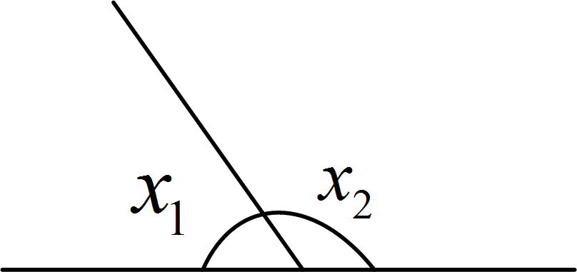
${{x}_{1}}+{{x}_{2}}={{180}^{\centerdot }}$
10. The angle by which the locus enters a complex zero is determined by the 180-degree criteria.
11.There is a limited stability where the root locus crosses the imaginary axis.
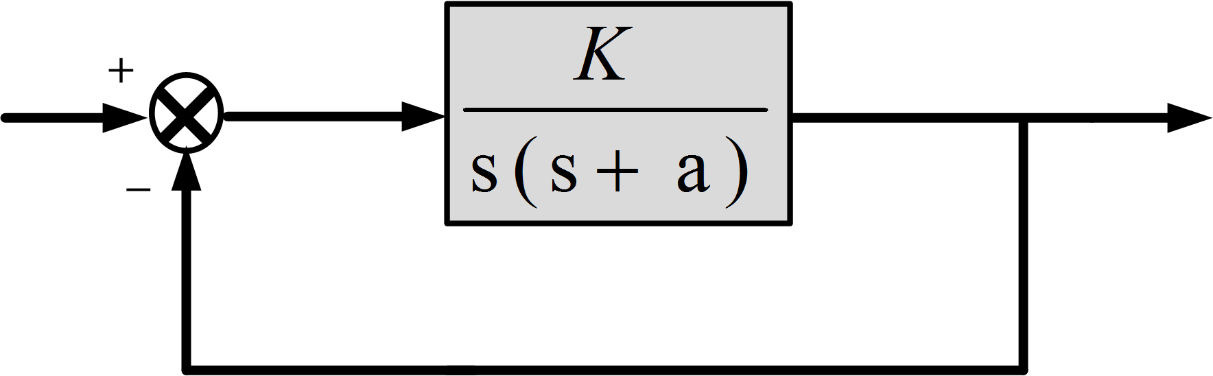
Root Locus Example
Find the loci of the closed-loop system poles for the following system
First, the open-loop pole-zero pattern is plotted, consisting of poles at the origin and at -a, as shown in the figure:
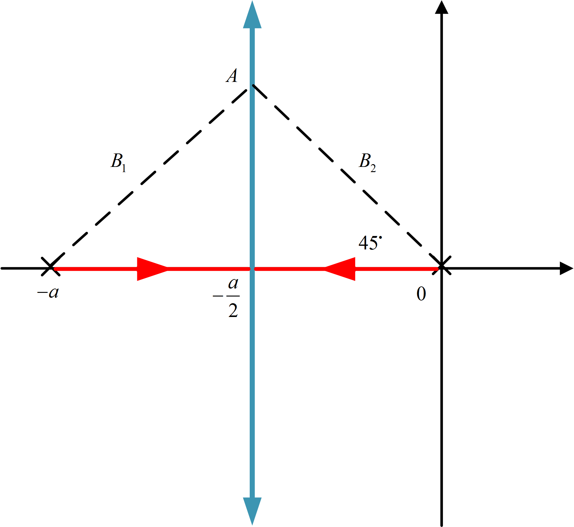
There are two poles, so two-locus branches, starting at 0 and -1 for K=0.
Since there are no open-loop zeros, there must be two asymptotes, from guideline 6, they will be at +90o and -90o.
From guideline 7, these asymptotes will intersect the real axis at
\[{{\sigma }_{A}}=\frac{0-a-0}{2-0}=-\frac{a}{2}\]
By guideline 3, the real axis between 0 and -a is part of the locus, because it lies to the left of one (an odd number) pole on this axis.
Root Locus Matlab
Now, we will talk about root locus using Matlab. Here, we will draw the root locus of the following transfer function:
\[GH(s)=\frac{s+2}{s(s+1)}\]
This is an open loop transfer function, however, in order to plot Root Locus (as we mentioned in the beginning), we need Closed-Loop Transfer Function Poles, which we can obtain from the following characteristic equation:
\[1+KGH(s)=1+K\frac{s+2}{s(s+1)}=0\]
The characteristics equation can be re-written as:
${{s}^{2}}+(1+K)s+2K=0$
Now, we will use the coefficients of the above characteristic equation in order to plot the Locus using Matlab.
Root Locus Plot Matlab Code
% Matlab Code to Compute Root Locus
% for 1 + K(s+2)/(s(s+1))
clear all; close all;clc

% Numerator and Denumerator for Open Loop Transfer Function
num = [1 2]; den = [1 1 0];
%Display Open-Loop Transfer Function
disp(['L(s) = ', poly2str(num,'s'), '/', poly2str(den, 's')]);
disp(' ');

figure

%Open-Loop Zeros, Plot with o's
olzeros = roots(num)
%Open-Loop Poles, Plot with x's
olpoles = roots(den)

% Plotting Open-Loop Zeros and Poles
plot(real(olzeros),imag(olzeros),'ro'); hold on;
plot(real(olpoles),imag(olpoles),'rx');

% Plot Closed-Loop Poles over Various Values of K
for K = 0.1:0.1:10,
 % Root of Characteristics Equation "1+KGH(s)"
 closed_poles = roots([1, 1+K, 2*K]);
 plot(real(closed_poles),imag(closed_poles),'bx');
end
hold off;
xlabel('Real Axis');
ylabel('Imaginary Axis');
title('Root Locus for Closed Loop Transfer Function');
Result
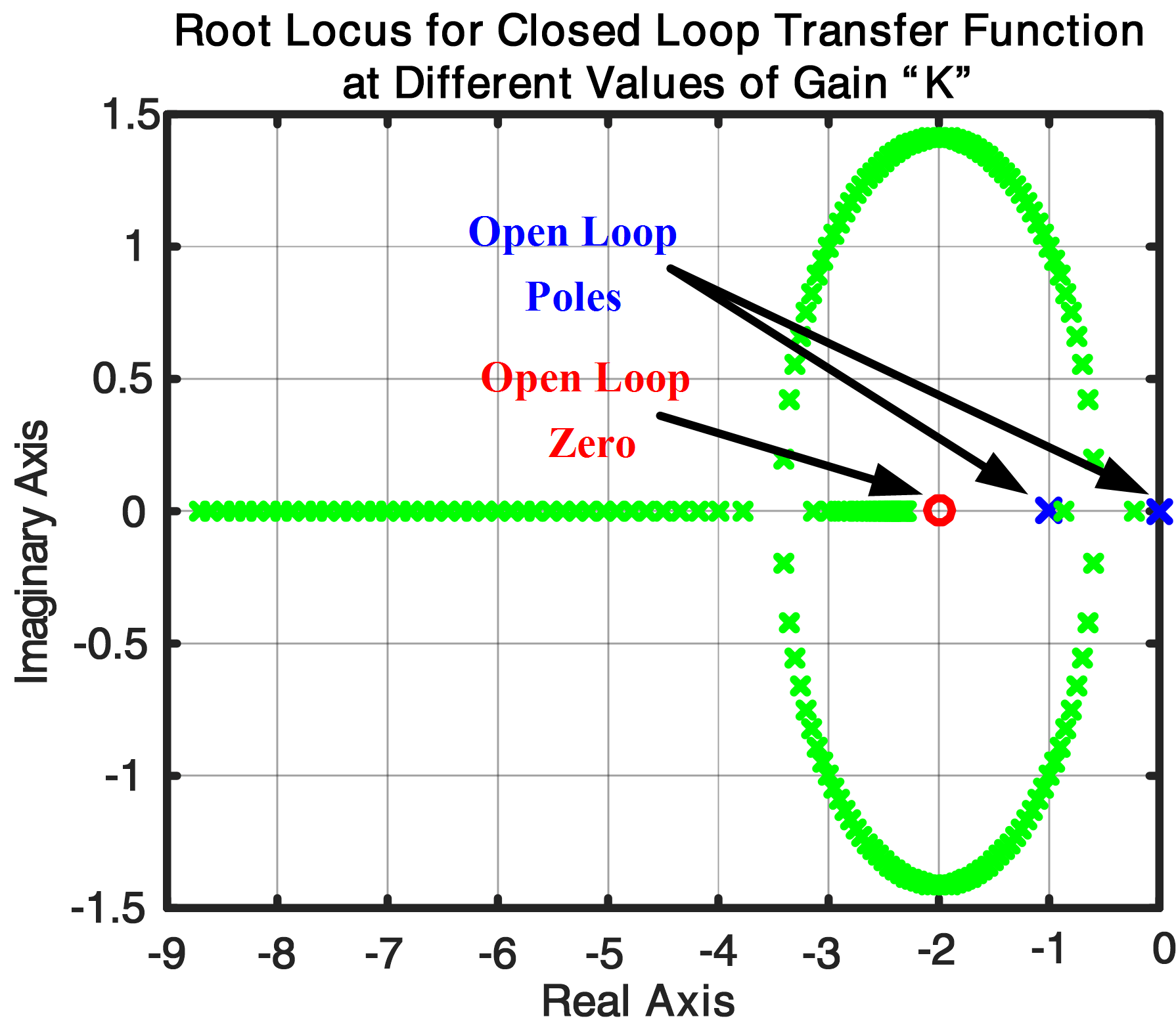
Figure: Root Locus for Closed-Loop Transfer Function at Various Values of Gain K
The above root locus graph shows the Open Loop transfer function Poles ( at -1 and 0 with blue *) and Zeros (at -2 with red o) as well as Closed Loop transfer function Poles at varying values of gain parameter K from 0.01 to 10.
Key Takeaways
Understanding the Root Locus method is essential for engineers and control system designers because it provides a powerful visual insight into how system poles—and consequently, system behavior—change with varying gain values. This technique is crucial for assessing and ensuring the stability and performance of feedback control systems. With the ability to predict system responses, design controllers, and fine-tune parameters effectively, Locus plays a vital role in applications ranging from industrial automation to robotics and aerospace engineering.