The article discusses steady-state error in feedback control systems, emphasizing the role of system type and gain in determining the accuracy of output tracking for different input signals. It outlines how higher system types and loop gains help reduce steady-state errors for step, ramp, and acceleration inputs.
Steady State Error
High loop gains were shown advantageous to reduce the sensitivity to modeling accuracy, parameter variations, and disturbance inputs. They will now prove equally desirable from the point of view of the reduction of steady-state errors in feedback systems.
Consider the unity feedback system in Figure 1. The transform of the error is
E=R-C
Where
C=GE
So,
\[E=\frac{R}{\left( 1+G \right)}\]
The steady-state error ess can be found directly, without the need for inverse transformation, by the final-value theorem:
${{e}_{ss}}=\underset{t\to \infty }{\mathop{\lim \text{ }}}\,e(t)=\underset{s\to 0}{\mathop{\lim }}\,\text{ }sE(s)=\underset{s\to 0}{\mathop{\lim }}\,\text{ }\frac{sR(s)}{1+G(s)}$ (1)
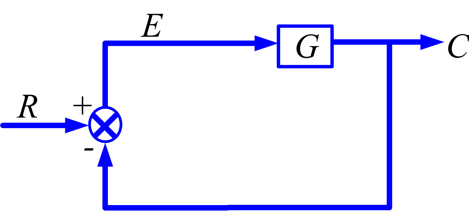
Figure 1: Unity Feedback System
For G(s), the following general form is assumed:
\[\begin{matrix} G(s)=\frac{K}{{{s}^{n}}}\frac{{{a}_{k}}{{s}^{k}}+\cdots +{{a}_{1}}s+1}{{{b}_{k}}{{s}^{k}}+\cdots +{{b}_{1}}s+1} & \cdots & (2) \\\end{matrix}\]
Definitions
Gain: K as given, with the constant terms in the numerator and denominator polynomials made unity, is formally the gain of the transfer function G and can be expressed as:
$gain\text{ K=}\underset{s\to 0}{\mathop{\lim }}\,\text{ }{{\text{s}}^{\text{n}}}\text{G(s)}$
Type number: the type number of G is the value of the integer n. A factor s in the denominator represents an integration, so the type number is the number of integrators in G.
Position error Constant Kp: the value of gain K for n=0
Velocity error Constant Kv: the value of gain K for n=1
Acceleration error Constant Ka: the value of gain K for n=2
These three special names of the gain are often used.
Equation (2) shows that
$\underset{s\to 0}{\mathop{\lim }}\,\text{ G(s)=}\underset{s\to 0}{\mathop{\lim }}\,\text{ (}\frac{K}{{{s}^{n}}}\text{)}$
So (1) can be written as
\[{{e}_{ss}}=\underset{s\to 0}{\mathop{\lim }}\,\text{ }\frac{sR(s)}{1+({}^{K}/{}_{{{s}^{n}}})}\]
This readily yields Table 1 for the steady-state errors corresponding to different type numbers and inputs. For example, for a type 2 system with a unit ramp input,
\[{{e}_{ss}}=\underset{s\to 0}{\mathop{\lim }}\,\text{ }\frac{s({}^{1}/{}_{{{s}^{2}}})}{1+({}^{K}/{}_{{{s}^{2}}})}=\underset{s\to 0}{\mathop{\lim }}\,\frac{s}{{{s}^{2}}+K}=0\]
Table 1 Steady-State Errors
Input n=0 n=1 n=2
Step u(t), R=1/s $\frac{1}{1+{{K}_{p}}}$ 0 0
Ramp t, $R=\frac{1}{{{s}^{2}}}$ ∞ $\frac{1}{{{K}_{v}}}$ 0
Acceleration $\frac{{{t}^{2}}}{2}$ , $R=\frac{1}{{{s}^{3}}}$ ∞ ∞ $\frac{1}{{{K}_{a}}}$
For insight into these results, it is useful to consider Figure 2, which shows type 0 and type 1 systems for s→∞. for n=0, C=KpE, so there cannot be a nonzero output without a proportional nonzero error, if the output must increase along a ramp, the error must increase according to a ramp as well. So a type 0 has a steady-state error for a step input and cannot follow a ramp,
For n=1,
$C=\frac{{{K}_{v}}}{s}E\text{ }$
so,
$\text{c(t)=}{{\text{K}}_{\text{v}}}\int{e(t)dt}$
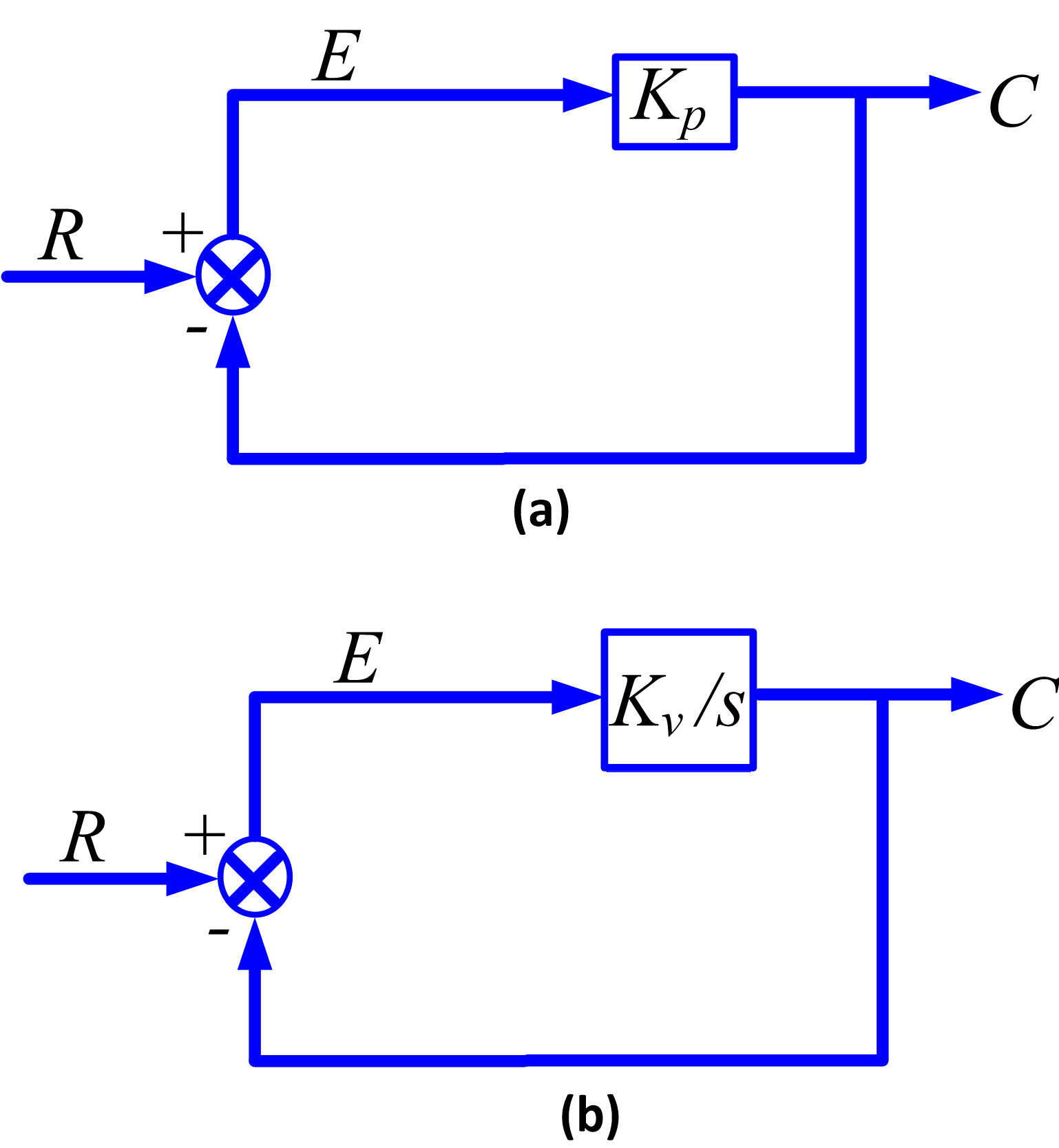
Figure 2: Type (a) 0 and (b) 1 systems
Therefore, the output cannot level off to a constant value unless the error levels off at zero. A steady state with nonzero steady state error cannot exist for a step input because the integrator would cause the output to change. This means that if, as is often the case, the performance specifications require zero steady-state error after a step input, and the designer must ensure that the system is at least of type 1. A type 2 system would be necessary if zero steady-state errors following both steps and ramps were specified.
The nonzero finite errors in Table 1 decrease as the gain is increased, as do parameter sensitivity and disturbance response. For larger K, a smaller error can attain the same effect on the output.
Steady State Error Key Takeaways
In practical applications, minimizing steady-state error is crucial for ensuring accurate and stable performance in systems such as robotics, aerospace, and industrial automation. Understanding system type and gain helps engineers design controllers that meet precision requirements, maintain consistent tracking of desired inputs, and enhance overall reliability despite disturbances or parameter variations.