This article explores the concept of Signal Flow Graphs, their components, and definitions, alongside an in-depth explanation of Mason’s Gain Formula, which simplifies the calculation of system transfer functions, complete with an illustrative example to demonstrate its application.
What is a Signal Flow Graph?
A Signal Flow Graph (SFG) is a graphical representation of a system that illustrates the relationships between its variables using nodes and directed branches. Each node represents a system variable, such as an input, output, or intermediate variable, while the branches indicate the functional dependency between these variables, labeled with corresponding transfer functions or gains.
An SFG is primarily used in control systems and signal processing to analyze and simplify complex linear systems by systematically applying Mason’s Gain Formula to compute the system’s transfer function, which relates the input and output variables. It is a powerful analytical tool that enables visualization of system dynamics, providing insights into feedback loops, forward paths, and system stability.
The application of mason’s gain formula to the signal flow graph corresponding to a given detailed block diagram is undoubtedly simplest operational procedure for obtaining the system transfer function. A signal flow graph is composed of various loops and one or more paths leading from an input to an output. Nodes representing system variables are interconnected by branches. Some important definitions and properties related to signals flow graph are given below:
Node. A node represents a system variable in the signal flow graph. It can denote an input, output, or intermediate variable in the system. Nodes are connected by branches to illustrate their interdependencies.
Branch. A branch is a directed line connecting two nodes in the SFG. It represents the relationship between the connected variables, with the branch gain denoting the proportionality factor or transfer function between the nodes.
Input Node. An input node is a node in the graph that has only outgoing branches. It represents the external input to the system.
Output Node. An output node is a node that has only incoming branches. It represents the final output of the system.
Path. A path is any continuous sequence of branches in the graph where all arrows point in the same direction. It connects one node to another without revisiting any node.
Loop. A loop is a closed path that starts and ends at the same node without visiting any node more than once (except for the starting/ending node). It represents feedback in the system.
Common Node. A common node is a node that belongs to two or more loops. It is where the loops share a connection point.
Non-Touching Loops. Non-touching loops are loops in the graph that do not share any common nodes. They are entirely independent of each other.
Forward Path. A forward path is a directed path from an input node to an output node that does not pass through any node more than once. It represents a unique route from input to output without revisiting any variable.
Gain. Gain is the product of the branch gains along a path or loop. For a path, it is the cumulative effect of all transfer functions from the starting node to the ending node. For a loop, it represents the feedback gain around the loop.
These terms collectively provide the building blocks for analyzing systems using signal flow graphs, allowing for the systematic application of tools such as Mason’s Gain Formula to determine system transfer functions and dynamics.
Mason’s Gain Formula
Mason’s Gain Formula is a method used to determine the transfer function of a system represented by a signal flow graph (SFG). It provides a way to calculate the overall gain from the input to the output of a system, accounting for both forward paths and feedback loops.
The formula is particularly useful for systems with multiple feedback loops and forward paths, where traditional block diagram reduction techniques might become cumbersome. It simplifies the process of handling complex systems with interconnected loops and paths.
Mason’s gain formula is composed of three types of terms:
1. We identify all forward paths and designate the path gains as Pk for k=1,2,3,…
2. We form a parameter ∆ which denotes the interactions among the various loops.
∆=1 – (sum of all single loops gains) + (sum of products of gains of all possible combinations of two non-touching loops) – (sum of products of gains of all possible combinations of three non-touching loops) + ….
3. We form a parameter ∆k (for k=1,2,3,…) Which is a cofactor of kth forward path, obtained from ∆ by removing the loops that touch this path.
So mason’s gain formula for the overall gain is
$$T = \frac{1}{\Delta} \sum_{k=1}^{N} P_k \Delta_k$$
Signal Flow Graph Example
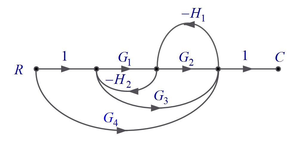
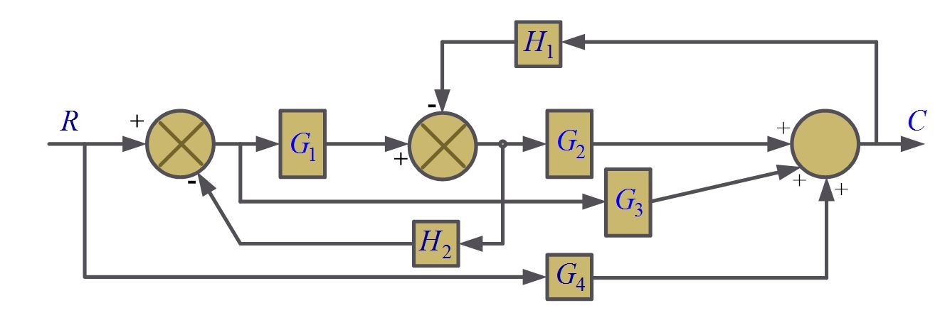
1. There are three forward paths from R to C and three loops, with gains
${{P}_{1}}={{G}_{1}}{{G}_{2}}$
${{P}_{2}}={{G}_{3}}$
${{P}_{3}}={{G}_{4}}$
${{L}_{1}}=-{{G}_{1}}{{H}_{2}}$
${{L}_{2}}=-{{G}_{2}}{{H}_{1}}$
${{L}_{3}}={{G}_{3}}{{H}_{1}}{{H}_{2}}$
2. All three loops touch, so ∆ is 1 minus sum of the loop gains
$\Delta =1-(-{{G}_{1}}{{H}_{2}}-{{G}_{2}}{{H}_{1}}+{{G}_{3}}{{H}_{1}}{{H}_{2}})$
$\Delta =1+{{G}_{1}}{{H}_{2}}+{{G}_{2}}{{H}_{1}}-{{G}_{3}}{{H}_{1}}{{H}_{2}}$
3. Special Case
If all forward paths and all loops touch each other, it may be seen that the cofactors are all unity.
In this example, the forward paths P1 and P2 touch all three loops so the corresponding cofactors ∆1 and ∆2 are unity. However, loop L1 does not touch path P3 so;
${{\Delta }_{3}}=1+{{G}_{1}}{{H}_{2}}$
Substituting values from above all three steps into the mason’s gain formula yields the closed loop transfer function.
$$T=\frac{{{P}_{1}}{{\Delta }_{1}}+{{P}_{2}}{{\Delta }_{2}}+{{P}_{3}}{{\Delta }_{3}}}{\Delta }$$
So,
$$T=\frac{{{G}_{1}}{{G}_{2}}+{{G}_{3}}+{{G}_{4}}(1+{{G}_{1}}{{H}_{2}})}{1+{{G}_{1}}{{H}_{2}}+{{G}_{2}}{{H}_{1}}-{{G}_{3}}{{H}_{1}}{{H}_{2}}}$$
Mason’s gain formula is preferable to determine transfer function either directly for simple systems or with the use of digital computers for large-scale systems having many feedback loops and forward paths.