Capacitive Reactance
The AC Current flow in a capacitor depends on the supply voltage and the capacitive reactance. The capacitance value and the supply frequency determine the capacitive reactance.
The alternating current through a capacitor leads the capacitor terminal voltage by 90o as shown in the figure below.
If a sinusoidal voltage is applied to a pure capacitance ( no series or parallel resistance), the current is maximum when the voltage begins to rise from zero.one-quarter a cycle later, the current is zero when the voltage across the capacitor is maximum. This condition, illustrated in figure 1, shows that the current waveform leads the applied emf by 90o.
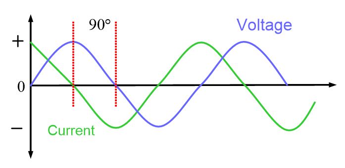
Fig.1: Current and Voltage in a Capacitive Circuit
- You May Also Read: Inductive Reactance
Capacitive current flow depends on the size of the capacitor and the rate of charge and discharge. At higher frequencies, the rate of charge and discharge increases per unit time. For a purely capacitive circuit, the charging current is as follows:
$i=\omega CV$
Capacitive reactance (XC)
Opposition to the flow of an alternating current by the capacitance of the circuit; equal to ${}^{1}/{}_{2\pi fC}$ and measured in ohms.
The ratio of effective voltage across the capacitor to the effective current is called the capacitive reactance and represents the opposition to current flow. Its symbol is XC and is measured in ohms. Mathematically, capacitive reactance is expressed as follows:
${{X}_{C}}=\frac{1}{2\pi fC}\text{ }\cdots \text{ (2)}$
Where
f=frequency in hertz
C=capacitance in farads
Example
What is the reactance of an 8 μF filter capacitor at 120 Hz?
Solution
${{X}_{C}}=\frac{1}{2\pi fC}=\frac{1}{2\pi *120*8*{{10}^{-6}}}=165.87\Omega $
Graph of XC
Equation (2) indicates there is an inverse relationship between capacitance and frequency and a capacitor’s reactance. That is, as the former two increase, the latter decreases. See the graph in figure 2.
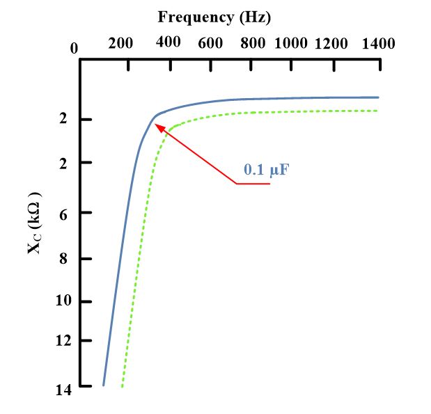
Fig.2: Graph of XC vs Frequency
Note that XC is shown in the fourth quadrant, opposite XL, which is in the first quadrant. St very low frequencies, approaching dc, the reactance increases at a rapid rate. At DC, the denominator of equation (2) would be zero and the reactance infinite. As the frequency increases, the reactance becomes smaller, approaching 0 Ω at very high frequencies.
As is evident from figure 2, the curve represents the reactance characteristics of 0.1 μF capacitor. For other capacitor values, the curve assumes slightly different shapes. If the capacitance is reduced, the curve moves towards the right (dotted line); for increased capacities, it moves toward the left. In other words, the solid curve shown represents the varying reactance characteristics of 0.1 μF capacitor only.
XC in Series and Parallel
Series and parallel combinations of capacitive reactance are treated in the same manner as inductive reactance. Therefore, the total reactance of two or more series-connected capacitors is as follows:
${{X}_{CT}}={{X}_{{{C}_{I}}}}+{{X}_{{{C}_{2}}}}+\cdots +{{X}_{{{C}_{n}}}}$
Two parallel capacitive reactances have the following total reactance:
${{X}_{CT}}=\frac{{{X}_{{{C}_{I}}}}{{X}_{{{C}_{2}}}}}{{{X}_{{{C}_{I}}}}+{{X}_{{{C}_{2}}}}}$
Which is the familiar product-over-sum formula. If three or more capacitors are parallel-connected, their net reactance is as follows:
$\frac{1}{{{X}_{CT}}}=\frac{1}{{{X}_{{{C}_{1}}}}}+\frac{1}{{{X}_{{{C}_{2}}}}}+\frac{1}{{{X}_{{{C}_{3}}}}}+\cdots +\frac{1}{{{X}_{{{C}_{n}}}}}$
Currents and voltages experienced around the capacitive circuit are calculated by using Ohm’s law, where XC is substituted for R. the following example illustrates the procedure.
Example
Using the circuit of figure 3, Calculate ${{X}_{CT}},\text{ }{{\text{I}}_{\text{T}}}\text{, }{{\text{V}}_{{{\text{C}}_{\text{1}}}}}\text{, and }{{\text{V}}_{{{\text{C}}_{\text{2}}}}}$ .
Solution
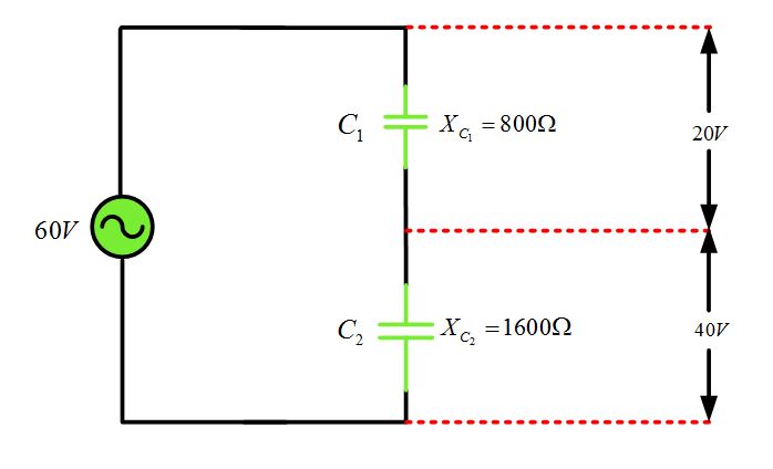
Fig.3: Circuit of the Example
${{X}_{CT}}={{X}_{{{C}_{1}}}}+{{X}_{{{C}_{2}}}}=800+1600=2400\Omega $
${{I}_{T}}=\frac{E}{{{X}_{CT}}}=\frac{60}{2400}=25mA$
${{V}_{{{C}_{1}}}}={{I}_{T}}{{X}_{{{C}_{1}}}}=25*800=20V$
\[{{V}_{{{C}_{2}}}}={{I}_{T}}{{X}_{{{C}_{2}}}}=25*1600=40V\]
Clearly, the voltage drops are proportional to the series reactances.
Example
Using the circuit of figure 4, Calculate ${{X}_{CT}},\text{ }{{\text{I}}_{{{C}_{1}}}}\text{, }{{\text{I}}_{{{C}_{2}}}}\text{, and }{{\text{I}}_{\text{T}}}$ .
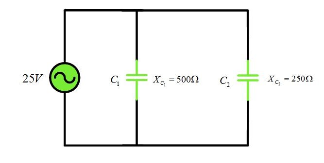
Fig.4: Circuit of the Example
Solution
${{X}_{CT}}=\frac{{{X}_{{{C}_{I}}}}{{X}_{{{C}_{2}}}}}{{{X}_{{{C}_{I}}}}+{{X}_{{{C}_{2}}}}}=\frac{500*250}{500+250}=167\Omega $
${{I}_{{{C}_{1}}}}=\frac{25}{500}=50mA$
${{I}_{{{C}_{2}}}}=\frac{25}{250}=100mA$
${{I}_{T}}={{I}_{{{C}_{1}}}}+{{I}_{{{C}_{2}}}}=50+100=150mA$
Clearly, the current flows are inversely proportional the reactance values.
Capacitive Susceptance
The reciprocal of capacitive reactance XC is capacitive susceptance BC, which is a measure of purely capacitive circuit’s ability to pass current.
The capacitive susceptance formula can be expressed as:
\[{{B}_{C}}=\frac{1}{{{X}_{C}}}\]