Conductors carry electric current. Insulators protect conductors and protect people from conductors. Whether a material is a conductor or an insulator depends on its atoms and on the relationship of each atom to its surrounding atoms.
Insulators may break down if subjected to excessive voltages. Similarly, conductors may be destroyed if too much current is passed through them. The best conductor materials have the lowest resistivity, that is, resistance per cubic meter. The best insulator materials have the highest breakdown voltage for a given thickness.
The resistance of any conductor can be calculated from a knowledge of its cross-sectional area, its length, and the resistivity of the material. Once the resistance is known, the voltage drop along a conductor and the power dissipated in it can be determined for any given current.
Insulators
Figure 1 shows some typical arrangements of conductors and insulators. Electric cable usually consists of conducting copper wire surrounded by an insulating sheath of rubber or plastic. Sometimes there is more than one conductor, and these are, Of course, individually insulated.
Fig. 1: Conductors and Insulators
Conductors employed for industrial and domestic purposes normally have stranded copper wires with rubber or plastic insulation. In electronic equipment, flat cables of fine wires and thin printed circuit conductors are widely used.
Even in the best of insulating materials, there are some free electrons drifting about between the atoms. Therefore, a very small electric current can flow through an insulator. In normal circumstances, this current is so small that it is absolutely negligible. A current can also flow along the surface of an insulator, especially if the insulator is dirty or wet. This is particularly evident with the porcelain insulators on high-voltage overhead cables during a rainstorm, when arcing occurs over the insulator surface.
If a sufficiently high potential difference is applied across an insulator, electrons can be pulled out of the atoms, and substantial current flow may occur. This is known as an insulator breakdown, and it normally results in the destruction of the insulator. To help avoid breakdown, all insulating materials are rated according to the maximum voltage that may be safely applied. Table 1 lists typical breakdown voltages (or dielectric strengths) for various insulating materials. It is seen that the air has the lowest breakdown voltage, at 30 kV/cm, and mica has the highest, at 2000 kV/cm.
The electric field strength is a measure of the electric stress set up in an insulator. The field strength should always be lower than that which might cause insulator breakdown. The field strength is simply the applied voltage divided by the insulator thickness.
$\begin{matrix} \text{electricfield strength,}\xi \text{=}\frac{E}{d} & {} & \left( 1 \right) \\\end{matrix}$
Where E is in volts and d is in meters, the unit of field strength is volts/meter (V/m). The situation is illustrated in figure 2 and further explored in the following example.
Table.1: Typical breakdown voltages of some insulating materials
| Material | Breakdown voltage (kV/cm) |
| Air | 30 |
| Porcelain | 70 |
| Rubber | 270 |
| Glass | 1200 |
| Mica | 2000 |
Fig.2 (a): Two Conductor Cable
Fig.2 (b): Cable Cross-Section
Conductors and Insulators Example
Two electric conductors encased in rubber are exactly 0.25 cm apart.
(a). Calculate the electric field strength in the insulation when the potential difference between the conductors is 25 V.
(b). Determine the minimum potential difference between conductors and insulators breakdown.
Solution
From equation (1)
$\text{electricfield strength,}\xi \text{=}\frac{E}{d}=\frac{25}{0.25}=100V/cm$
From table 1, insulation breakdown for rubber occurs at 270 kV/cm.
$E\text{=}d\times \text{breakdown voltage=0}\text{.25*270=67}\text{.5kV}$
Conductors
The function of a conductor is to conduct current from one point to another in an electric circuit. Electric cables usually consist of copper conductors sheathed with rubber or plastic insulating material. Cables that have to carry large currents must have relatively thick conductors. Where very small currents are involved, the conductors may be a thin strip of copper or even an aluminum foil. Between these two extremes, a wide range of conductors exists for various applications. Three different types of cables used in electronics equipment are illustrated in Figure 3. The one identified as a coaxial cable has a central insulated conductor and a circular plaited conducting screen, as well as an outer insulating sheath. The other two are multi-conductor cables, one circular, and one flat.
Fig.3: Different types of cables
Many different types of cables are used with electronics equipment.
Because each conductor has a finite resistance, a current passing through it causes a voltage drop from one end of the conductor to the other (Figure 4). When conductors are long and/or carry large currents, the conductor voltage drop may cause unsatisfactory performance of the equipment supplied. Power (I2R) is also dissipated in every current-carrying conductor, and this is, of course, wasted power.
Fig.4 (a): Current Flow through a conductor produces a voltage drop

Fig.4 (b): Conductor resistance causes voltage drop
Conductor resistance (R) is determined by applying the voltage drop and current level to Ohm’s law. The resistance per unit length (R/l) is then used to select a suitable wire gauge.
In extreme cases, the power dissipated in the conductors may generate sufficient heat to destroy the insulation or even melt the conductor. Where the resistance per unit length of a conductor is known, the conductor voltage drop and power dissipation are easily calculated.
To select a conductor for a given application, its resistance per unit length is first determined from the current level and the acceptable voltage drop along the cable. The table is then used to find a wire gauge with the calculated resistance per kilometer (R/km) or with the next lower R/km value.
Conductor Resistivity
The resistance per unit length of a given conductor is not always available. Therefore, to allow for all possible combinations of cable length and cross-sectional area. The specific resistance of the conducting material is employed.
The specific resistance (or resistivity) of a material is the resistance of 1-meter cube of the material.
Obviously, as some metals are better conductors than others, each has its own specific resistance. Table 2 lists the specific resistances of venous metals.
The symbol used for specific resistance is ρ (Greek lowercase letter rho), and the units of p are ohm meters (Ωm).
Consider the meter cube of copper illustrated in Figure 5 (a). From Table 2, the specific resistance of copper is p =1.72 X 10⁻⁸ Ωm.
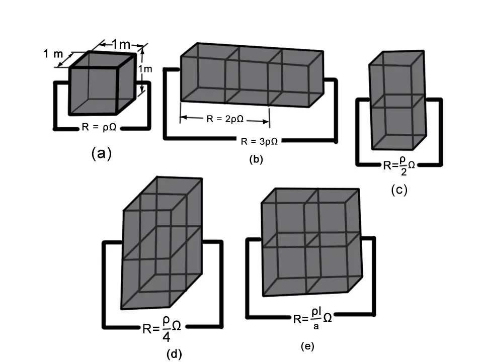
Fig.5: Block Resistances
If a 1-meter cube of copper has a resistance of ρ Ω, three cubes in series will have a resistance of 3 ρ Ω, and the resistance of two in parallel will be ρ/2 Ω.
If the length of copper is doubled or tripled by placing blocks side by side as shown in Figure 5(b), the resistance is increased. (Blocks or other components, connected together in this way are said to be connected in series. The resistance of two series-connected blocks is 2p Ω and that of three is 3p Ω, and so on. From this, it is derived that the total resistance of any length of copper with a cross-sectional area of 1 m2 is,
$\begin{align} & R=\rho \times (\text{length in meters}) \\ & =1.72*{{10}^{-8}}\times (\text{length in meters) }\Omega \\\end{align}$
Now consider the effect of doubling the cross-sectional area of the copper by placing two blocks as illustrated in Figure 5 (c). (Blocks or other components, connected together in this way are said to be connected in parallel. Because the cross-sectional area is doubled, the resistance is halved. If four blocks are parallel-connected [Figure 5 (d)] the resistance is quartered. In the case of blocks connected in parallel, the resistance can be written as,
\[R=\frac{\rho }{\text{cross-sectional area in }{{\text{m}}^{\text{2}}}}\]
Table.2: Specific resistance for electrical conducting metals
| Metal | Specific resistance at 20 oC (Ωm) |
| Silver | 1.64*10-8 |
| Copper | 1.72*10-8 |
| Gold | 2.45*10-8 |
| Aluminum | 2.83*10-8 |
| Tungsten | 5.5*10-8 |
| Nickel | 7.8*10-8 |
When blocks are put in series and parallel [Figure 5(e)], the two previous equations are combined to give
\[\begin{matrix} R=\rho \frac{l}{a} & {} & \left( 2 \right) \\\end{matrix}\]
Where R is the resistance in ohms, p is the specific resistance of the material, l is the length in meters, and a is the cross-sectional area in m2.
Cylindrical shaped conductors with different dimensions are illustrated in Figure 6. It is seen that the resistance of a conductor with length l1 and cross-section a1 is calculated as
\[{{R}_{1}}=\rho \frac{{{l}_{1}}}{{{a}_{1}}}\]
Fig.6: Conductors Resistance for different lengths
Conductor resistance is determined by the length, cross-sectional area, and the specific resistance of the conductor material.
A similar conductor with the same cross-sectional area and twice the length has a resistance of 2R1. Also, a conductor with the same length as the first but a cross-sectional area of 2a has a resistance of R1/2.
The resistance of any length of a conductor of any cross-sectional area can be calculated from equation (2). Where R, l, and a are known, the equation can be rewritten to determine the specific resistance:
Example
Determine the resistance of 20 m of annealed copper wire 2 mm in diameter.
Solution
Cross sectional area:
\[a=\frac{\pi {{D}^{2}}}{4}=\frac{\pi {{\left( 2\times {{10}^{-3}} \right)}^{2}}}{4}=\pi \times {{10}^{-6}}{{m}^{2}}\]
From equation (2)
\[R=\rho \frac{l}{a}\]
From table 2, for Copper
$\rho =1.72*{{10}^{-8}}$
Therefore,
\[R=1.72\times {{10}^{-8}}\times \frac{20}{\pi \times {{10}^{-6}}}=0.109\Omega \]
The resistance of any conductor can be calculated from a knowledge of its cross-sectional area, its length, and the resistivity of the material. Once the resistance is known, the voltage drop along a conductor and the power dissipated in it can be determined for any given current.
Temperature Effects on Conductors
The values of specific resistance stated in Table 2 refer only to conducting materials at a temperature of 20oC. Thus, in all resistance calculations using the specific resistance, the conductor temperature is assumed to remain constant at 20oC. Because the resistance of metals changes with temperature, it is necessary to be able to calculate the resistance values at higher or lower temperature levels.
The resistance of all pure metals tends to increase as the temperature of the metal rises. This may be explained in terms of the atoms actually vibrating at elevated temperatures and, thus, becoming greater obstructions in the path of moving electrons. Because the resistance increases with increasing temperatures, metals are said to have a positive temperature coefficient (PTC). Some materials, notably semiconductors, exhibit a decrease in resistance as their temperature rises. These have a negative temperature coefficient (NTC). Over the normal range of operating temperatures, all metals exhibit a nearly linear relationship between resistance and temperature.
In Figure 7(a) the variation in resistance of copper is plotted versus temperature. Note that the resistance of copper appears to go to zero at a temperature of -234.5oC. The actual graph is not as completely linear as illustrated, however, the straight line passing through -234.5oC is a projection of the linear portion of the graph. If the resistance R1 at a temperature of 20oC is known, the new value of resistance at any other temperature can be calculated.
Fig.7 (a): Resistance of Copper plotted versus Temperature
Suppose that R1 is 1 Ω at 20oC. If the temperature is reduced to -234.5oC, the temperature change is
\[\Delta T={{20}^{o}}C-\left( -{{234.5}^{o}}C \right)={{254.5}^{o}}C\]
And the resistance change per degree of temperature change is
\[\frac{\Delta {{R}_{1}}}{\Delta T}=\frac{1}{254.5}=0.00393{\Omega }/{^{o}C}\;\]
If R1 were 10 Ω (instead of 1 Ω) at 20oC, the resistance change with temperature would be
\[\frac{\Delta {{R}_{1}}}{\Delta T}=\frac{10}{254.5}=0.0393{\Omega }/{^{o}C}\;\]
The quantity 0.00393 Ω/oC is the temperature coefficient for copper at 20oC.
The symbol α or (Greek lowercase letter alpha) is used for temperature coefficient. Table 3 lists the temperature coefficients for various metals at 20oC. Note that the alloy constantan has an extremely small temperature coefficient. This characteristic makes constantan useful in applications where resistance is required to remain as constant as possible when the temperature changes. Temperature coefficients can also be determined at temperatures other than 20oC. Column 3 in table 3 lists temperature coefficients at 0oC.
Table.3: Temperature coefficients for metals
| Material | α at 20oC | α at 0oC |
| Silver | 0.003 8 | 0.004 12 |
| Copper | 0.003 93 | 0.004 26 |
| Gold | 0.003 4 | 0.004 65 |
| Aluminum | 0.003 9 | 0.004 24 |
| Tungsten | 0.004 5 | 0.004 95 |
| Nickel | 0.006 | |
| Constantan | 0.000 008 |
Fig. 7 (b): The resistance (R2) at a new temperature (T2) can be determined from a knowledge of R1 and T1 and the temperature coefficient α
As explained, for any conducting material having a resistance R1,
\[\frac{\Delta {{R}_{1}}}{\Delta T}=\alpha {{R}_{1}}\]
Or
$\begin{matrix} \Delta {{R}_{1}}=\alpha {{R}_{1}}\Delta T\text{ } & \cdots & [\text{ see Figure 7 (a) and (b) }] \\\end{matrix}$
And resistance R2 at a new temperature T2 is
$\begin{matrix} {{R}_{2}}={{R}_{1}}+\Delta {{R}_{1}}={{R}_{1}}+\alpha {{R}_{1}}\Delta T\text{ } & {} & [\text{ see Figure 7 (b) }] \\\end{matrix}$
Therefore,
$\begin{matrix} {{R}_{2}}={{R}_{1}}\left( 1+\alpha \Delta T \right) & {} & \left( 3 \right) \\\end{matrix}$
Where R1 is the resistance at 20oC, α is the temperature coefficient of the material, and ∆T is the temperature change from 20oC.
If R1 and R2 are known, equation (3) can be rearranged to determine ∆T or α:
\[\Delta T=\frac{1}{\alpha }\left( \frac{{{R}_{2}}}{{{R}_{1}}}-1 \right)\]
\[\alpha =\frac{1}{\Delta T}\left( \frac{{{R}_{2}}}{{{R}_{1}}}-1 \right)\]
The temperature coefficient at 0oC may also be used in equation (3) if the resistance R1 is measured at 0oC and ∆T is the temperature increase from 0oC.
Conductors and Insulators Key Takeaways
In summary, conductors and insulators play crucial roles in electrical and electronic applications. Conductors ensure efficient transmission of electrical current, while insulators provide protection, preventing unwanted current flow and ensuring safety. The understanding of resistance, breakdown voltages, and material properties is essential for designing electrical circuits, power transmission systems, and electronic devices. Choosing the right conductor or insulator based on specific requirements—such as resistivity, voltage rating, and environmental conditions—optimizes performance and prevents failures.