The article discusses the behavior of an AC circuits containing resistance and inductance, explaining the phasor relationships between voltage and current, Kirchhoff’s voltage law, and the addition of sine-wave voltages. It introduces the phasor diagram, phasor addition (geometric and algebraic), and the use of complex numbers for simplifying AC circuit analysis in the frequency domain.
Figure 1 shows a simple AC circuits containing resistance and inductance. The sine-wave voltage source causes a sine wave of current to flow in the circuit. Since all the components are connected in series, the current in the inductance and the current in the resistance must have the same magnitude at every instant.
In fact, the sine-wave currents in the inductance and the resistance are one and the same thing, so we can represent both with the letter symbol i.
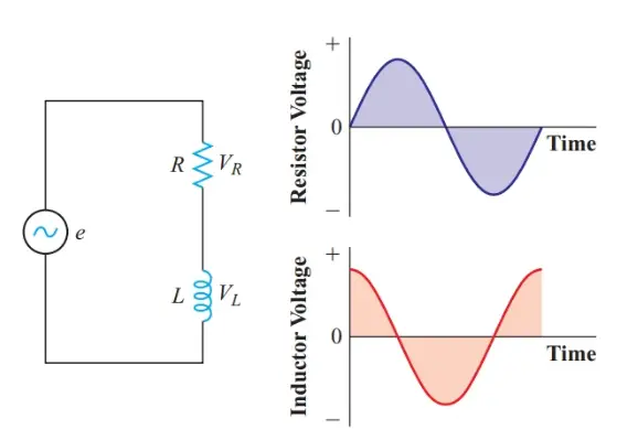
Figure 1 AC circuit with resistor and inductor in series
The sine wave of current through the resistance causes a sine-wave voltage drop across it that is exactly in phase with the current sine wave.
The instantaneous current through inductance lags behind the instantaneous voltage applied to it by π/2 radians. Consequently, the sine-wave voltage across the inductance and the sine-wave voltage across the resistance are π /2 radians out of phase, and the instantaneous voltage across the inductance reaches its positive peak π /2 radians earlier than the instantaneous voltage across the resistance.
Kirchhoff’s voltage law states that the sum of the voltage drops in a series circuit must equal the applied voltage. In DC circuits where the source voltage is independent of time, we can find the sum of the voltage drops by simple arithmetic.
Now we need to find the sum of two out-of-phase sine-wave voltages. We can represent a sine-wave voltage either by its instantaneous value, v = Vm sin ωt or by its RMS value, V = 0.707 Vm.
Since the instantaneous value varies continuously and depends on the elapsed time, it is said to belong to the time domain. In the time domain, we express the angular distance traveled by a sine wave in radians. We can use ordinary algebra for calculations with instantaneous values.
Since the RMS value of a sine wave does not vary with the exact instant in time, we treat a sine-wave alternating voltage as a phasor quantity having a magnitude and a phase angle. Such quantities are said to belong to the frequency domain. Calculations with phasors require a specialized form of algebra, which is described later in the chapter.
Addition of Instantaneous Values
Since Kirchhoff’s voltage law applies to the circuit in Figure 1 at every instant,
\[\begin{matrix}e={{v}_{T}}={{v}_{R}}+{{v}_{L}} & {} & \left( 1 \right) \\\end{matrix}\]
Therefore, we can add the instantaneous values of sine waves by simple arithmetic addition. Although the sum of the instantaneous voltages at one instant does not give us the overall picture of the addition of complete sine waves, we can repeat the calculation at intervals over a complete cycle to determine the nature of the resultant wave.
To help with this time-consuming task, we can draw the sine curves for the two sets of instantaneous values on the same graph, as in Figure 2. Since angular velocity is constant for a given frequency, we can show the phase angle of the source, ωt, instead of time on the horizontal axis.
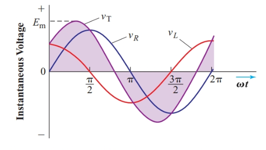
Figure 2 Addition of two out-of-phase sine waves
At t = 0, the instantaneous voltage across the resistance is zero; therefore, the instantaneous value of the total voltage is the same as the voltage across the inductance at that instant.
As time elapses, the instantaneous voltage across the inductance is decreasing and the instantaneous voltage across the resistance is increasing. At approximately 1 rad, their sum reaches its peak value. At π /2 rad, the instantaneous voltage across the inductance is zero, and the instantaneous value of the total voltage equals the instantaneous voltage across the resistance.
Approximately 1 rad later, the instantaneous values of the voltages across the resistance and the inductance are equal in magnitude but opposite in polarity, so vT = 0.
Careful examination of Figure 2 shows that the waveform for vT is a sine wave with the same period as vR and vL. In fact, any sum of sine waves with the same frequency has this property.
The sum of sine waves of the same frequency is also a sine wave of the same frequency.
Equation 1 can be expanded to
\[\begin{matrix}e={{V}_{mR}}\sin \omega t+{{V}_{mL}}\sin \left( \omega t+{}^{\pi }/{}_{2} \right) & {} & \left( 2 \right) \\\end{matrix}\]
Since vR and vL do not reach their peak values at the same instant, the peak value of vT occurs at a time when the instantaneous values of the two-component voltages are less than their peak values. Therefore,
\[{{E}_{m}}\ne {{V}_{mR}}+{{V}_{mL}}\]
Since the RMS value of any sine wave equals the peak value divided by$\sqrt{2}$,
\[E\ne {{V}_{R}}+{{V}_{L}}\]
Therefore, arithmetic addition does not apply to peak and RMS values if the sine waves are out of phase, as in Figure 2. However, if the sine waves are exactly in phase, as in Figure 3, the resultant and component sine waves do reach their peak values at the same instant, and
\[\begin{matrix}{{E}_{m}}={{V}_{m1}}+{{V}_{m2}} & and & E={{V}_{T}}={{V}_{1}}+{{V}_{2}} \\\end{matrix}\]
Thus, the RMS value of the sum of in-phase sine waves is simply the sum of the RMS values of the individual sine waves.
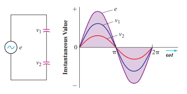
Figure 3 Addition of instantaneous values of two in-phase sine waves
Representing a Sine Wave by a Phasor Diagram
Once we accept that the addition of sine waves of the same frequency results in a sine wave of the same frequency, the tedious procedure required to produce Figures 2 and 3 is not warranted. The original information from which we constructed those graphs was simply their RMS values and the phase angle between them. RMS value and phase angle will also serve to identify the resultant.
If we draw phasors for the two sine-wave voltages in the circuit of Figure 1, the rotating phasor for the instantaneous voltage across the inductance will always stay exactly p/2 radians ahead of the rotating phasor for the instantaneous voltage across the resistance. Consequently, these voltage phasors do not move in relation to each other.
Sine waves of the same frequency can be represented by “stationary” phasors with the angle between the phasors representing the phase angle between the sine waves.
When drawing phasors for electrical quantities, we make the length of the phasors proportional to the RMS value of the sine wave they represent. These AC phasors belong to the frequency domain, where angles are usually expressed in degrees.
In the simple series circuit of Figure 1, the current is common to all components. Therefore, in the phasor diagram for a series AC circuit, such as in Figure 4, we draw a phasor representing the RMS value of the current along the reference axis of the diagram (pointing toward three o’clock).
Since the voltage across the resistance is in phase with the current through it, the phasor VR points in the same direction as the current phasor. Since the voltage across the inductance leads the current through it by 90°, we orient VL 90° counterclockwise from the reference axis.
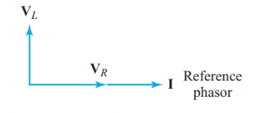
Figure 4 Phasor diagram for the AC Circuit of Figure 1
The phasor diagram of Figure 4 is much easier to draw than the instantaneous voltage graphs of Figure 2, and it shows the RMS values and phase angles at a glance.
Letter Symbols for Phasor Quantities
In studying the behavior of electric and magnetic circuits, we encounter three types of quantities.
Scalers
Scalars are quantities that have magnitude but no direction or angle. Resistance, inductance, and capacitance are scalars. Voltage and current in DC circuits are scalars, as are instantaneous values of voltage and current in AC circuits. Scalars are represented by lightface italic letter symbols (such as R, L, C, V, I, v, and i). Scalar quantities can be added by simple algebraic addition.
Vectors
Vectors are quantities that have both magnitude and direction. Electrostatic force, electric field intensity, and magnetic flux density are all vector quantities.
This article uses boldface italic letter symbols (such as F, E, and B) to represent vector quantities, and the same letter symbols in lightface italic to represent magnitudes of vectors. For example, the magnitude of the vector F is the scalar quantity F.
Most electric vector quantities have three dimensions. However, if all the vectors for a particular calculation lie in the same plane, we can treat them as being two-dimensional. Because vectors are multidimensional, most operations in vector algebra, such as addition and multiplication, differ substantially from the simple arithmetic operations for scalars.
Phasors
Phasors are quantities that have both magnitude and direction. Phasor notation is a convenient method for representing sine waves in AC circuits. For example, a sine-wave voltage can be represented as V =V∠ϕ, where V is the RMS magnitude and ϕ is the phase angle.
We use bold Roman letters for phasors to distinguish them from vectors, shown by bold italic letters. As with vectors, the same letter in lightface italic indicates the magnitude of a phasor.
Using phasor notation we can rewrite Equation 2 as
\[\begin{matrix}{{\text{E}}_{\text{T}}}\text{=}{{\text{V}}_{\text{R}}}\text{+}{{\text{V}}_{\text{L}}} & {} & \left( 3 \right) \\\end{matrix}\]
Phasor Addition by Geometrical Construction
In a phasor diagram, the resultant of two phasor quantities is the diagonal from the origin to the opposite corner of the parallelogram with the two phasors as sides.
The resultant can be constructed with ruler and compass, as shown in Figure 5. Using a radius equal to the length of E1, we trace an arc with the tip of the E2 phasor as the center. Next, using a radius equal to the length of E2, we trace an arc with the tip of E1 as the center. We then draw the resultant by joining the origin to the intersection of the two arcs.
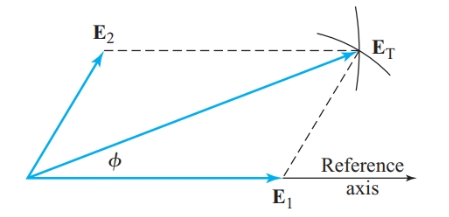
Figure 5 Geometrical construction of a resultant phasor
Applying this technique to the series circuit of Figure 1 shows how the magnitudes and phase angles of E, I, VR, and VL are related. Figure 6 compares the sine-wave graph and the phasor diagram for this series circuit. Although we can determine RMS values and phase angles from the sine-wave graphs in Figure 6(a), it is much easier to get this information from the phasor diagram in Figure 6(b).
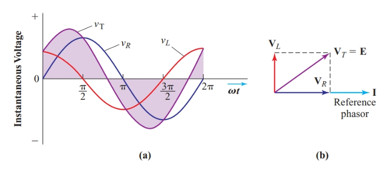
Figure 6 Sine-wave graph and phasor diagram for the circuit of Figure 1
If we draw the phasors carefully, we can measure the RMS voltages and the phase angle between the applied voltage E and the current I to two-figure accuracy. Although graphical solutions are not accurate enough for many of the AC circuit problems, we can use approximate values from a phasor diagram to check the calculated answers.
Phasor diagrams also help us to get the correct sign for the sine, cosine, or tangent of angles larger than 90°.
Phasor Addition of Perpendicular Phasors
Earlier, we saw that the RMS values of sine waves that are in phase can be added arithmetically. Therefore, phasors that have the same phase angle can be simply added together. Similarly, when the angle between a pair of phasors is exactly 180°, the phasor sum is simply the difference of the two phasors. For two phasors with an angle of exactly 90° between them, we can use trigonometry to find the phasor sum.
In the simple series circuit of Figure 1, the voltage drop across the resistance is exactly in phase with the current and the voltage across the inductance leads the current by exactly 90°. Therefore, the two voltage phasors are exactly 90° out of phase. In the geometrical construction for their resultant in Figure 8(a), the parallelogram becomes a rectangle with side AC exactly equal to the magnitude of the VL. Therefore, the triangle in Figure 8(b) shows exactly the same data as the conventional phasor diagram of Figure 8(a), which has all the phasors starting from the origin. Such triangular diagrams are useful for analyzing AC circuits that have both resistance and reactance.
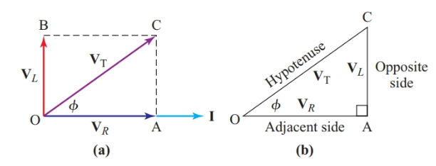
Figure 8 Addition of phasors at right angles
Since triangle OAC is a right triangle,
\[\tan \phi =\frac{opposite\text{ side}}{adjacent\text{ side}}=\frac{AC}{OA}=\frac{{{V}_{L}}}{{{V}_{R}}}\]
Given the RMS voltages across the inductance and the resistance, we can find the phase angle ϕ using trigonometric tables or a calculator with a tan–1 function.
\[\begin{matrix}\phi ={{\tan }^{-1}}\frac{{{V}_{L}}}{{{V}_{R}}} & {} & \left( 4 \right) \\\end{matrix}\]
Where tan–1 means “the angle having a tangent of.”
We now have a choice of several methods for finding the magnitude of the total voltage, ET. From trigonometry,
\[\sin \phi =\frac{opposite\text{ side}}{hypotenuse}=\frac{AC}{OC}\]
Therefore,
\[\begin{matrix}{{E}_{T}}=\frac{{{V}_{L}}}{\sin \phi } & {} & \left( 5 \right) \\\end{matrix}\]
Similarly,
\[\cos \phi =\frac{\text{adjacent side}}{hypotenuse}=\frac{OA}{OC}\]
Therefore,
\[\begin{matrix}{{V}_{T}}=\frac{{{V}_{R}}}{\cos \phi } & {} & \left( 6 \right) \\\end{matrix}\]
Another method uses the Pythagorean Theorem, which states that the square of the length of the hypotenuse of a right triangle is equal to the sum of the squares of the lengths of the other two sides. In Figure 8(b),
\[O{{C}^{2}}=O{{A}^{2}}+A{{C}^{2}}\]
\[\begin{matrix}{{V}_{T}}=\sqrt{V_{R}^{2}+V_{L}^{2}} & {} & \left( 7 \right) \\\end{matrix}\]
Note that it is customary to state the resistance component before the reactive component in Equation 7. Combining Equations 7 and 4 gives
\[\begin{matrix}{{E}_{T}}=\sqrt{V_{R}^{2}+V_{L}^{2}}\angle {{\tan }^{-1}}\frac{{{V}_{L}}}{{{V}_{R}}} & {} & \left( 8 \right) \\\end{matrix}\]
Expressing Phasors with Complex Numbers
When we describe a phasor by stating its magnitude and phase angle with respect to the reference axis, we are using polar coordinates. These coordinates specify the position of the tip of the phasor in terms of a distance along a radius from the origin and an angle measured from the reference axis.
Polar coordinates correspond to the measurements we obtain with instruments such as voltmeters, ammeters, and wattmeters.
By applying trigonometric relationships to the phasor diagram of Figure 8, we determined the polar coordinates of the total voltage from two perpendicular components, one of which lies along the reference axis. We can use the same method to find rectangular coordinates (or perpendicular components) for any phasor in the polar form E∠ϕ.
As shown in Figure 9, the reference axis component (or real component) is the magnitude of the phasor multiplied by the cosine of its phase. The quadrature component (or imaginary component) is the magnitude of the phasor multiplied by the sine of its phase angle.
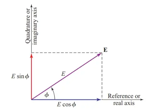
Figure 9 Determining the rectangular coordinates of a phasor
The rectangular coordinates of a phasor indicate distances along the axes of the complex plane. Figure 10 shows how angles in polar coordinates correspond to the four possible directions for coordinates in the complex plane.
In the complex plane, multiplying a phasor by the j operator rotates it 90° counterclockwise. To rotate the phasor another 90°, we simply multiply once more by the j operator. Hence, multiplying a phasor by j2 changes its direction by 180°.
In polar coordinates, reversing the direction of a phasor is the same as multiplying by –1. Hence j2=–1. Since $j=\sqrt{-1}$ has no solution, numbers preceded by the +j or –j operator are called imaginary numbers. Multiplying a phasor by j three times rotates it a total of 270°. Since j3 = j2 × j and j2 = -1, the operator –j corresponds to a rotation of 270°.
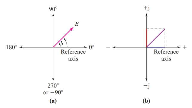
Figure 10 Corresponding directions in (a) polar coordinates and (b) rectangular coordinates
The rectangular coordinates of a phasor consist of a real number (which can be positive or negative) and an imaginary number identified by either +j or –j. The real component is always listed before the imaginary component. The formula for converting a voltage phasor from polar coordinates to rectangular coordinates is
\[\begin{matrix}E\angle \phi =+E\cos \phi +jE\sin \phi & {} & \left( 9 \right) \\\end{matrix}\]
This equation demonstrates how any sine wave quantity can be expressed in terms of a complex number that has real and imaginary components.
Equation 8 indicates a procedure for converting from rectangular coordinates to polar coordinates. The magnitude of the polar quantity is simply the square root of the sum of the squares of the rectangular coordinates, leaving out the j operator. We find the phase angle by drawing a diagram of the perpendicular components. The angle between the phasor and its reference axis component is
\[\theta ={{\tan }^{-1}}\frac{quadrature\text{ }coordinate}{reference\text{ }axis\text{ }coordinate}\]
We then use the diagram to determine the actual phase angle with respect to the reference axis.
Phasor Addition Using Rectangular Coordinates
Although there are trigonometric procedures for adding phasors having angles between them of other than 0° or 90°, it is usually much easier to express the phasors in rectangular coordinates and then find the sum of the components.
Since all the real components of the phasors are horizontal, we can simply add them algebraically. Similarly, the imaginary components are all vertical, so we can also add them algebraically. These two sums are the real and imaginary components of the resultant phasor. All that remains is to convert these rectangular coordinates into polar form. This procedure is the conventional method of phasor addition for AC circuit problems.
Subtraction of Phasor Quantities
When two phasors are expressed in rectangular coordinates, one can be subtracted from the other by simple algebraic subtraction of first the real (or reference axis) components and then the imaginary (or quadrature) components. The resulting rectangular coordinates can then be converted into polar form.
Multiplication and Division of Phasor Quantities
Multiplication and division of phasor quantities in polar form is the simplest of all the complex algebra processes.
To multiply quantities expressed in polar form, multiply their magnitudes and add their phase angles algebraically.
\[\begin{matrix}{{E}_{1}}\times {{E}_{2}}={{E}_{1}}\angle {{\phi }_{1}}\times {{E}_{1}}\angle {{\phi }_{2}}={{E}_{1}}{{E}_{2}}\angle {{\phi }_{1}}+{{\phi }_{2}} & {} & \left( 10 \right) \\\end{matrix}\]
To divide phasor quantities expressed in polar form, divide their magnitudes and subtract their phase angles algebraically.
\[\begin{matrix}{{E}_{1}}\div {{E}_{2}}={{E}_{1}}\angle {{\phi }_{1}}\div {{E}_{1}}\angle {{\phi }_{2}}=\frac{{{E}_{1}}}{{{E}_{2}}}\angle {{\phi }_{1}}-{{\phi }_{2}} & {} & \left( 11 \right) \\\end{matrix}\]
Although the procedure for multiplying and dividing phasor quantities expressed in rectangular coordinates is straightforward, it does require skill in manipulating algebraic terms. It is often safer to do phasor multiplication and division by the simpler polar method.
With a calculator that has coordinate-conversion functions, such conversions are the quickest way to do phasor multiplication and division.
Phasor Diagram and Phasor Algebra Key Takeaways
- The sum of two sine waves having the same frequency is also a sine wave of the same frequency.
- The peak value of the sum of two sine waves having the same frequency is not the sum of their peak values unless the sine waves are in phase.
- The polar coordinates of a phasor give its magnitude and phase angle.
- The rectangular coordinates of a phasor give the values of its real and imaginary components.
- Phasors may be added or subtracted on a phasor diagram.
- Phasors may be added or subtracted when expressed in rectangular coordinates.
- Phasors are simpler to multiply or divide when they are expressed in polar coordinates.