The article introduces the Bode Plot, a graphical representation of the frequency response of a system, with separate plots for magnitude and phase. It explains the advantages of Bode Plots, the concept of corner frequency or breakpoint, and details the construction of Bode Plots for various elementary factors like gain factor, integrator, differentiator, simple lag, simple lead, and quadratic factor (second order). The MATLAB code for generating Bode Plots for these factors is provided along with corresponding plots. Additionally, the article discusses special terms related to Bode Plots and their significance in analyzing the stability of a system.
What is a Bode Plot?
H.W. Bode introduced a method to present the information of a polar plot of a transfer function GH(s), actually the frequency response GH (jω), as two plots with the angular frequency were at the common axis. The first plot shows the magnitude of the transfer function as a function of ω, and the second plot shows the phase as a function of ω. This pair of plots is referred to as Bode Plot or Bode Diagram.
The magnitude of the transfer function is expressed in decibels (dB), the phase in degrees and the common parameter of frequency is plotted on a logarithmic scale in radians. At times, the magnitude of a transfer function is referred to as gain and the corresponding plot as a gain plot.
Bode Plot Advantages
- One apparent advantage of the bode diagram is the relative ease with which it is obtained.
- A second advantage is that this technique is feasible for lower frequencies, where measuring the phase difference between input and output signals is difficult.
- A third advantage results from the introduction of logarithms, thus reducing the process of multiplying two transfer functions to addition.
Corner frequency or Breakpoint
In the bode-plot, low-frequency asymptote (that is ω<<1/T) and high-frequency asymptote (that is ω>>1/T) cut off at 0 decibels (dB) line where ω=1/T, that is the frequency called corner frequency or break point.
Matlab Bode Plots
The Bode plot or diagram of a transfer function can be constructed by combining the transfer functions of the following elementary factors.
- Gain factor K
- Integrator or Differentiator
- Simple lag or simple lead
- Quadratic lag or quadratic lead
We will discuss the above elementary factors one by one:
Gain factor K
A constant K may be considered as complex number expressed in polar form with magnitude K and angle 0. if K is positive or -180. if K is negative. For gain factor K, the bode-plot is obtained as:
If the open loop gain is
$G\left( j\omega \right)H\left( j\omega \right)=K$
Then its Magnitude (dB) is
\[{{\left| G\left( j\omega \right)H\left( j\omega \right) \right|}_{dB}}=20log\left| K \right|=\text{Constant}\]
Its Phase is
\[\angle G(j\omega )H(j\omega )=\left\{ \begin{matrix} {{0}^{\centerdot }} & K>0 \\-{{180}^{\centerdot }} & K<0 \\\end{matrix} \right.\]
The value in decibels is positive when the magnitude of the constant is greater than 1 and negative when less than 1.A number equal to 1 has a value of 0 in decibels.
The log-magnitude plot for a gain factor K is a straight horizontal line with a magnitude of 20 logK decibels. By changing the value of gain K in the transfer function brings up or brings down the log-magnitude curve by the proportionate amount. The gain factor K has no effect on the phase curve of the bode plot.
Matlab Bode Plot for Constant Gain Factor K
Here, we implemented the bode plot of gain factor K for the comprehensive understanding of the readers.
% Bode Plot for Constant Gain Factors K=4,10,12

clear all;close all;clc

num1 = 4;

den = [1];

sys1 = tf(num1,den);

grid;

bodeplot(sys1)

hold on

num2 = 10;

den = [1];

sys2 = tf(num2,den);

grid;

bodeplot(sys2)

hold on

num3 = 20;

den = [1];

sys3 = tf(num3,den);

grid;

bodeplot(sys3)

grid on

hold off

legend('K=4','K=10','K=12','Orientation','horizontal');
Bode Plot for Gain Factor
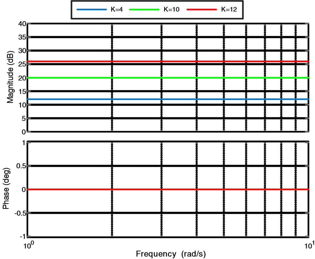
Figure 1. Bode Plot for Gain Factor K
Integrator and Differentiator
Pure integrator and differentiator are represented by transfer function 1/s and s respectively. Bode plots are obtained from the corresponding frequency response function 1/jω and jω.
For differentiator, the bode-plot is obtained as:
If the open loop gain is
$G\left( j\omega \right)H\left( j\omega \right)=j\omega $
Then its Magnitude (dB) is
\[{{\left| G\left( j\omega \right)H\left( j\omega \right) \right|}_{dB}}=20log\left| j\omega \right|=20log(\omega )\]
And it’s Phase is
\[\angle G(j\omega )H(j\omega )=\angle j\omega ={{90}^{\centerdot }}\]
When we draw a bode plot for a differentiator, we can observe that the magnitude plot is a straight line with a slope of +20 dB/decade. Whereas, the phase plot is a straight line with an angle of 90o.
Matlab Bode Plot for Differentiator
Here, we implemented the Bode plot of a differentiator for the comprehensive understanding of the readers.
% Bode Plot for Differentiator

clear all;close all;clc

% Transfer function

K = [1 0];

T = 1;

num = [K];

den = [T];

H = tf(num, den)

% Bode Plot

grid on

bode(H);
Bode Plot for Differentiator
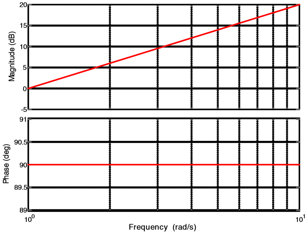
Figure 2. Bode Plot for Differentiator
Similarly, for Integrator, the bode-plot is obtained as:
If the open loop gain is
$G\left( j\omega \right)H\left( j\omega \right)={}^{1}/{}_{j\omega }$
Then its Magnitude (dB) is
${{\left| G\left( j\omega \right)H\left( j\omega \right) \right|}_{dB}}=20log\left| \frac{1}{j\omega } \right|=20log(1)-20log(\omega )=-20log(\omega )$
Its Phase is
\[\angle G(j\omega )H(j\omega )=\angle \frac{1}{j\omega }=-{{90}^{\centerdot }}\]
When we draw a bode plot for the integrator, we can observe that the magnitude plot is a straight line with a slope of -20 dB/decade. Whereas, the phase plot is a straight line with an angle of -90o.
Matlab Bode Plot for Integrator
Here, we implemented the bode plot of Integrator for the comprehensive understanding of the readers.
% Bode Plot for Integrator

clear all;close all;clc

% Transfer function

K = [1];

T = 1;

num = [K];

den = [T 0];

H = tf(num, den)

% Bode Plot

grid on

bode(H)
Bode Plot for Integrator
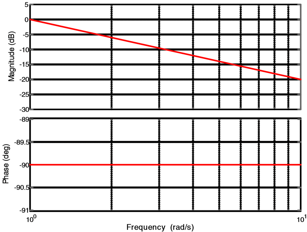
Figure 3. Bode Plot for Integrator
Simple lag or Simple Lead
These bode diagrams arise from phase-lag or phase-lead networks whose respective transfer functions are 1/Ts+1 and Ts+1.
For a simple phase-lag network, the bode-plot is obtained as:
If the open loop gain is
\[G\left( j\omega \right)H\left( j\omega \right)=\frac{1}{1+j\omega T}\]
Where T is a real constant.
Then its Magnitude (dB) is
\[{{\left| G\left( j\omega \right)H\left( j\omega \right) \right|}_{dB}}=20log\left| \frac{1}{1+j\omega T} \right|=20log\left| 1 \right|-20log\left| 1+j\omega T \right|=-20log(\sqrt{{{1}^{2}}+{{\omega }^{2}}{{T}^{2}}})\]
For Magnitude Plot
For low-frequency asymptote (when s→0)
When ω<<1/T (very very small, like approaches to zero), then the magnitude would be:
\[|G(j\omega )H(j\omega ){{|}_{dB}}=20\text{ }log(1)=0dB\]
This means that the magnitude plot would be a straight line at 0 dB at low frequency (ω<<1/T).
Similarly, for high-frequency asymptote (when s→∞)
When ω>>1/T (very very big, like approaches to infinity), then the magnitude would be:
\[|G(j\omega )H(j\omega ){{|}_{dB}}=-20\text{ }log(\omega T)\]
This means that the magnitude plot would be a straight line with -20 dB/decade slope at high frequency (ω>>1/T).
Its Phase is
\[\angle G(j\omega )H(j\omega )=\angle \frac{1}{1+j\omega T}=-{{\tan }^{-1}}(\omega T)\]
For Phase plot
When ω<<0.1/T, then
\[\angle G(j\omega )H(j\omega )={{0}^{\centerdot }}\]
This means that the phase plot would be a straight line at 0. until ω=0.1/T.
When ω=0.1/T, then
\[\angle G(j\omega )H(j\omega )=-{{45}^{\centerdot }}\]
This means that the phase plot would be a straight line with -45. /decade slope until ω=10/T.
When ω>>10/T, then
\[\angle G(j\omega )H(j\omega )=-{{90}^{\centerdot }}\]
This means that the phase plot would be a straight line at -90o.
Matlab Bode Plot for Simple Phase Lag Network
Here, we implemented the Bode plot of a Simple Phase Lag network for the comprehensive understanding of the readers.
% Bode Plot for Phase-Lag Network

clear all;close all;clc

% Transfer function

K = [1];

T = 1;

num = [K];

den = [T 1];

H = tf(num, den)

% Bode Plot

grid on

bode(H)

grid
Bode Plot for Simple Phase Lag Network
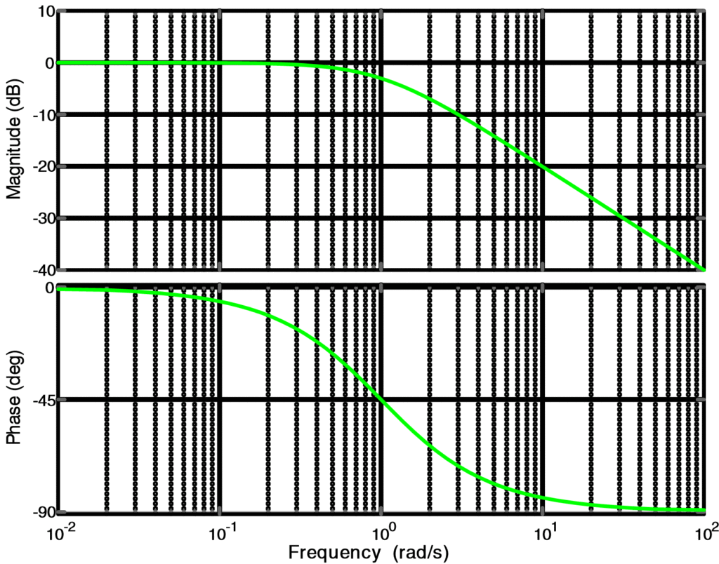
Figure 4. Bode Plot for Simple Phase-Lag Network
Similarly, for a simple phase-lead network, the bode-plot is obtained as:
If the open loop gain is
$G\left( j\omega \right)H\left( j\omega \right)=1+j\omega T$
Where T is a real constant.
Then its Magnitude (dB) is
\[{{\left| G\left( j\omega \right)H\left( j\omega \right) \right|}_{dB}}=20log\left| 1+j\omega T \right|=20log(\sqrt{{{1}^{2}}+{{\omega }^{2}}{{T}^{2}}})\]
For magnitude plot
For low-frequency asymptote (when s→0)
When ω<<1/T (very very small, like approaches to zero), then the magnitude would be:
\[|G(j\omega )H(j\omega ){{|}_{dB}}=20\text{ }log(1)=0dB\]
This means that the magnitude plot would be a straight line at 0 dB at low frequency (ω<<1/T).
Similarly, for high-frequency asymptote (when s→∞)
When ω>>1/T (very very big, like approaches to infinity), then the magnitude would be:
\[|G(j\omega )H(j\omega ){{|}_{dB}}=20\text{ }log(\omega T)\]
This means that the magnitude plot would be a straight line with +20 dB/decade slope at high frequency (ω>>1/T).
Its Phase is
\[\angle G(j\omega )H(j\omega )=\angle 1+j\omega T={{\tan }^{-1}}(\omega T)\]
For Phase plot
When ω<<0.1/T, then
\[\angle G(j\omega )H(j\omega )={{0}^{\centerdot }}\]
This means that the phase plot would be a straight line at 0. until ω=0.1/T.
When ω=0.1/T, then
\[\angle G(j\omega )H(j\omega )=-{{45}^{\centerdot }}\]
This means that the phase plot would be a straight line with +45. /decade slope until ω=10/T.
When ω>>10/T, then
\[\angle G(j\omega )H(j\omega )={{90}^{\centerdot }}\]
This means that the phase plot would be a straight line at 90o.
Matlab Bode Plot for simple Phase Lead Network
Here, we implemented the bode plot of a Simple Phase Lead network for the comprehensive understanding of the readers.
% Bode Plot for Phase-Lead Network

clc

% Transfer function

K = [1];

T = 1;

num = [K 1];

den = [T];

H = tf(num, den)

% Bode Plot

grid on

bode(H)

grid
Bode Plot for Simple Phase Lead Network
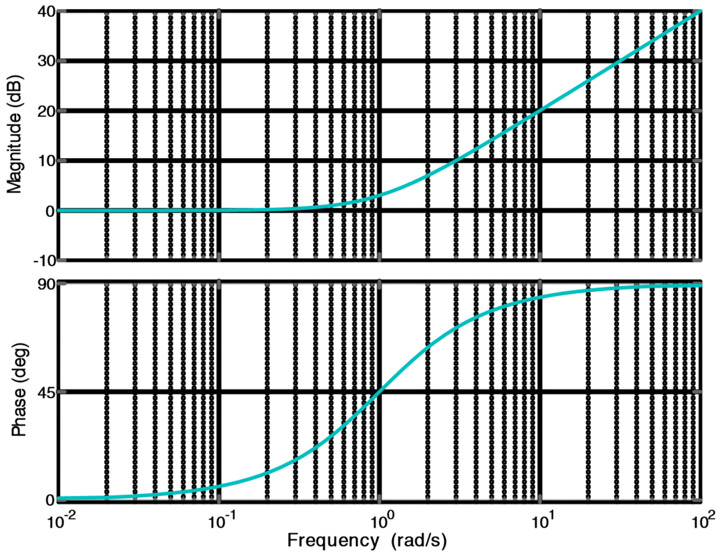
Figure 5. Bode Plot for Simple Phase-Lead Network
Quadratic Factor (Second Order)
The transfer function for a typical quadratic function can be written as
\[G\left( j\omega \right)H\left( j\omega \right)=\frac{\omega _{n}^{2}}{{{s}^{2}}+2\zeta {{\omega }_{n}}s+\omega _{n}^{2}}\]
The Magnitude Plot is obtained from
\[|G(j\omega )H(j\omega ){{|}_{dB}}=20\log \left| \frac{\omega _{n}^{2}}{{{\left( j\omega \right)}^{2}}+2\zeta {{\omega }_{n}}\left( j\omega \right)+\omega _{n}^{2}} \right|\]
\[|G(j\omega )H(j\omega ){{|}_{dB}}=20\log \left| \frac{1}{{{\left( {}^{j\omega }/{}_{{{\omega }_{n}}} \right)}^{2}}+2\zeta {{\omega }_{n}}\left( {}^{j\omega }/{}_{{{\omega }_{n}}} \right)+1} \right|\]
The above equation can be simplified as
\[|G(j\omega )H(j\omega ){{|}_{dB}}=-20~log{{\left[ {{\left( 1-{{\left( {}^{\omega }/{}_{{{\omega }_{n}}} \right)}^{2}} \right)}^{2}}+{{\left( {}^{2\zeta \omega }/{}_{{{\omega }_{n}}} \right)}^{2}} \right]}^{{}^{1}/{}_{2}}}\]
The Phase Plot is obtained from
\[\angle G(j\omega )H(j\omega )=-ta{{n}^{-1}}\left( \frac{{}^{2\zeta \omega }/{}_{{{\omega }_{n}}}}{1-{{\left( {}^{\omega }/{}_{{{\omega }_{n}}} \right)}^{2}}} \right)\]
In the above expression, the damping ratio ζ is a parameter and the frequency is normalized as ω/ ωn .
The bode-plot shown in the following figure was obtained from Matlab Software. Asymptotic approximations were drawn by two lines: one for a value of ω/ ωn <<1 and one for ω/ ωn >>1.
At low frequencies, that is, for values for ω such that ω<< ωn, the magnitude in decibels can be approximated by
\[|G(j\omega )H(j\omega ){{|}_{dB}}=-20\log {{1}^{{}^{1}/{}_{2}}}=0\]
Similarly, for higher frequencies that value of magnitude is approximated by
\[|G(j\omega )H(j\omega ){{|}_{dB}}=-20\log {{\left[ {{\left( -{{\left( {}^{\omega }/{}_{{{\omega }_{n}}} \right)}^{2}} \right)}^{2}} \right]}^{{}^{1}/{}_{2}}}=-40\log {}^{\omega }/{}_{{{\omega }_{n}}}\]
Which is a line with a slope of -40 dB/decade on semi-log paper. These asymptotes meet when ω= ωn =1; this point is called a break frequency or break point.
Similarly, for phase plot
When ω<< ωn , then
$\angle G(j\omega )H(j\omega )={{0}^{\centerdot }}$
This means that the phase plot would be a straight line at 0o.
When ω>> ωn , then
$\angle G(j\omega )H(j\omega )=-{{180}^{\centerdot }}$
This means that the phase plot would be a straight line at 180o.
When ω= ωn , then
$\angle G(j\omega )H(j\omega )=-{{90}^{\centerdot }}$
This means that the phase plot would be a straight line with -90. /decade slope.
Matlab Bode Plot for Second Order System
Here, we implemented the bode plot of a second-order network for the comprehensive understanding of the readers.
%Bode-Plot for Second-Order System

clear all;close all;clc

 fn = 1; % Define natural frequency (Hz)

 wn = 2*pi*fn; % Natural frequency conversion in rad/s

 Zeta = 0.05; % Damping Factor

 Num = [0 0 wn^2]; % Numerator

 Den = [1 2*Zeta*wn wn^2]; % Denominator

 Gs= tf(Num,Den) % Transfer Function

bode(Gs); %Bode-Plot

grid on
Bode Plot for Second Order System
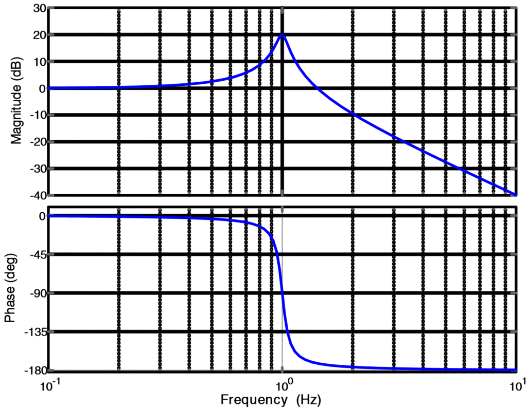
Figure 6. Bode Plot for Second Order System
Special Terms
There are certain terms, which we need to be familiar with to fully understand the bode plot.
Phase Cross-Over Frequency
It is the frequency, where phase shift becomes -180o.
Gain Cross Over Frequency
It is the frequency at which the amplitude ratio becomes 1 or the log modulus of the transfer function becomes 0.
Bode Plot and Stability
The characteristic equation of a typical system can be written as,
$1+GH\left( s \right)=0$
Where
$GH\left( s \right)=-1$
In the frequency domain,
$GH\left( j\omega \right)=-1$
How far -1 is from the open loop transfer function GH (jω) measures the stability of a system. This distance can be measured in terms called phase margin and gain margin.
Phase and gain margins are usually measured from open loop response and cannot be obtained from the frequency response of a closed loop system directly.
Gain Margin
It can be described as an increase in the open-loop system gain |GH (jω)| when the system phase is at 180. Which will cause marginal stability of a system.
In order to measure the gain margin,
- Find the point, where the system phase response crosses -180.
- At some point obtain amplitude response
- The distance below 0dB at this point shows the system gain margin.
Phase margin
In order to measure the phase margin,
- Find the point, where the system’s open-loop amplitude crosses 0 dB
- At some point, obtain the phase response
- The distance above -180. at this point shows the system phase margin
For a more comprehensive understanding, see the solved Example for Bode Plot using Matlab.
Bode Plot MATLAB Key Takeaways
Understanding and constructing Bode Plots is essential for engineers and system analysts because they offer a powerful visual tool for analyzing and designing control systems. The ability to graphically represent the frequency response through magnitude and phase plots helps in assessing system behavior, such as gain stability, phase margins, and bandwidth, which are critical for ensuring system performance and robustness. By breaking down complex transfer functions into simpler elementary factors—like gain, integrator, differentiator, and lag/lead components—Bode Plots make it easier to predict system responses to varying frequencies. This is particularly valuable in applications such as filter design, feedback loop tuning, and stability analysis in electrical, mechanical, and aerospace systems.
1 thought on “Bode Plot MATLAB | Bode Plot Transfer Function”