The article discusses the concepts of variable sampling and clock signals in microprocessor-controlled systems. It explains how analog data is converted to digital through periodic sampling and highlights the importance of sampling rate, sample-and-hold mechanisms, and the role of clock signals in synchronizing microprocessor operations.
In the processes or machinery that are controlled by a microcontroller or microprocessor, all analog data must be converted to digital, so that it can be represented by binary numbers and be usable by the microprocessor.
When a variable entity such as wind speed, car speed, or electric current in a motor is measured, the value obtained is for only the moment the measurement is performed. In a continuous process, the measured value is used for one or more necessary actions to be taken. For example, when a car is driven, the position of the gas pedal depressed by the driver is used to adjust car speed.
Sampling
In a continuous process, any measurement must be frequently repeated for updated values. Therefore, for microprocessor control of a device, another factor comes into the picture: the rate at which the data are updated. This updating of measured values is called sampling and how often a variable is updated is determined by the sampling rate.
The sampling rate can also be called sampling frequency, which implies how many times in one second the variable is measured. The time interval between every two measurements is called the sampling time.
For example, if in each second a variable is measured 1000 times, the sampling rate is 1000 per second, and the sampling time is 0.001 second. Depending on how important a role a parameter has in a process, this updating of values must be performed at a higher sampling rate.
Sampling: Action of measuring a variable in a process or machine repeatedly at a fixed frequency, for control purposes.
Sampling rate: Same as the sampling frequency. The (normally fixed) frequency at which a sampling action is performed.
Sampling frequency: The number of samples taken (or measurements made) in 1 second in a sampled data system. This is for converting analog values to digital values for digital control, computer control, display of values, and so on.
Sampling time: Time interval between every two consecutive measurements in a sampling action.
In Figure 1 a variable is sampled between times A and B. The variable is assumed to remain constant at the measured value for the total period of the sampling time until the next measurement is performed.
In reality, it is more likely that the value of variable changes even if the time interval is very small. For example, the value of the parameter at M is changing to that at N, whereas in the microcontroller it is kept constant until the new reading comes in, which implies a jump from N′ to N. It is thus obvious that more precision in measurement and control can be achieved by having a smaller sampling time. The measured value of any variable is stored by a circuit called sample and hold.
Sample and hold: Action of measuring a variable and storing the measured value for use. This is common in computer control systems where measurements are performed repeatedly (but not continuously; say at 1 msec intervals) at a properly fixed frequency.
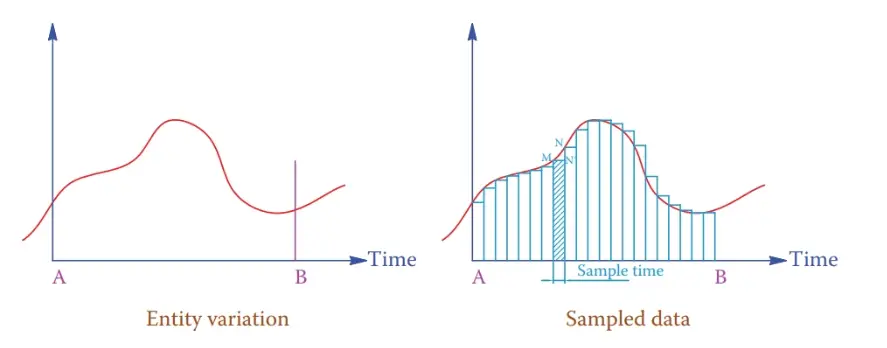
Figure 1 Sampling a variable parameter
Nowadays, fast sampling, for instance, one million samples per second (a sampling time of 1 microsecond) is possible for many measurements. This implies that the necessary time for measuring the variable under question, converting its value to digital and storing the result can be less than 1 millionth of a second. It must be noted that, in general, the higher the sampling rate is, the higher the price of the sampling equipment.
Increasing the sampling rate is not always necessarily essential, useful, or worth the cost even if possible. For example, consider the pitch angle of a wind turbine. If it takes 1 sec for the pitch angle to change (through its mechanism), any measurement faster than 1 per second does not have any useful effect. Also, if the measurement itself takes a long time, or the process is slow, such as heating a liquid, there is no point in sampling at a high rate. It can only add to the cost.
After sampling is performed at any instant, the measured value is converted to its binary form. This is repeated after each sampling time interval. Figure 2 shows a typical example of sampled data and its conversion to binary data (the binary conversion is only for demonstration).
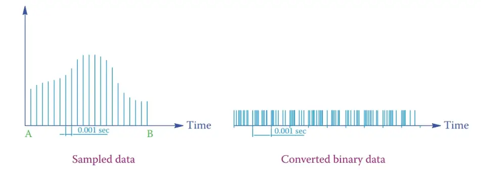
Figure 2 Sampled data and their binary conversion.
Clock Signal
Each microprocessor has a clock to regulate its operation. Each and every single operation, such as adding two bits of data, is performed with the clock pulse. Each clock pulse is a step for synchronized work of all components (for reading new values, conversions, mathematical operations, etc.) and all operations progress step by step.
A clock signal is a square pulse train with a fixed frequency. The clock rate can be decreased, and slower pulse trains are made from it for slower processes.
Figure 3 shows the pulse train of the clock signal and two other signals with half and one-quarter of the clock frequency. Each pulse has a rising edge, a falling edge, and a level part. A device can be sensitive to the rising edge or the falling edge, and, consequently, its function takes place with that part of a pulse. Some devices are level sensitive.
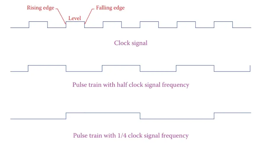
Figure 3 Representation of fixed frequency pulse signals.
A rising edge is also called a leading edge or a positive going edge. A falling edge is also called a trailing edge or a negative going edge. A pulse train continuously switches between zero and a positive value. We refer to these values as low and high.
Leading edge: Same as a rising edge in a square waveform.
Positive going edge: Rising edge in a square wave where the magnitude sharply goes positive from negative or zero.
Trailing edge: Same as a negative going edge, which is that edge of a rectangular waveform that the value drops from positive to negative or zero.
Negative going edge: Same as falling edge or trailing edge (changing from a positive value to a negative or zero value in a square wave).
Although microprocessors are very fast and their clock frequencies are in the range of MHz (million hertz), the change from a low level to a high level and vice versa is not instant, and, thus the time for switching (duration of the rising edge and falling edge) is not zero. In this sense, the actual clock signal and other signals are represented as shown in Figure 4.
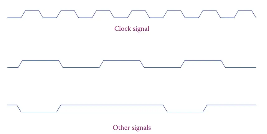
Figure 4 Representation of clock and other signals in a microprocessor.
Variable Sampling Key Takeaways
Understanding variable sampling and clock signals is crucial in microprocessor-controlled systems because they directly affect the accuracy, efficiency, and responsiveness of digital control processes. Sampling allows analog signals from real-world variables—like speed, temperature, or current—to be periodically converted into digital data for processing and decision-making. The sampling rate determines how accurately fast-changing variables can be tracked, while sample-and-hold circuits ensure the stability of measured values for precise computation. Clock signals, on the other hand, synchronize all operations within a microprocessor, ensuring orderly execution of tasks like data acquisition, conversion, and control actions. Together, these concepts form the foundation for reliable automation and control in applications such as automotive systems, industrial machinery, robotics, and home appliances—where timely, accurate data processing is essential for optimal performance.