The article discusses the modeling of a non-ideal transformer using an equivalent circuit that incorporates real-world characteristics like winding resistance, leakage flux, and core losses. It explains how these parameters are represented in both primary and secondary equivalent circuits, including their phasor forms and simplifications for practical analysis.
All transformers have winding resistance, a core with finite permeability, leakage flux, and hysteresis and eddy current losses and are thus non-ideal. These can be represented by an equivalent circuit that allows us to analyze the transformer.
Non-Ideal Transformer Characteristics
A non-ideal transformer is illustrated in Fig.1. It can be described by the following characteristics:
1. There is a flux leakage which means that not all of the flux produced by one winding will link the other winding.
2. Primary and Secondary windings have resistances which means that the applied voltage (source voltage) v1 is NOT the same as the induced primary voltage e1; that is, v1 ≠ e1. Similarly, v2 ≠ e2.
3. The magnetic core is NOT perfectly permeability which means that it requires a finite mmf for its magnetization.
4. Since the flux in the magnetic core is alternating, there exist hysteresis as well as eddy current losses, collectively called core or iron losses.
Equivalent Circuit of Transformer
In deriving the equivalent circuit for the two-winding transformer of Fig.1, the characteristics of an actual transformer described earlier need to be modeled.
Consider the primary circuit. A voltage equation around the loop may be written as
\[\begin{matrix} {{\nu }_{1}}={{R}_{1}}{{i}_{1}}+{{N}_{1}}\frac{d{{\lambda }_{1}}}{dt}={{R}_{1}}{{i}_{1}}+{{N}_{1}}\frac{d{{\phi }_{1}}}{dt} & {} & (1) \\\end{matrix}\]
Were
R1 = Resistance of primary winding
N1 = number of turns for primary winding
The primary winding flux ϕ1 may be expressed as the sum of the mutual flux ϕm and the primary leakage flux ϕ11:
$\begin{matrix} {{\phi }_{1}}={{\phi }_{m}}+{{\phi }_{11}} & {} & (2) \\\end{matrix}$
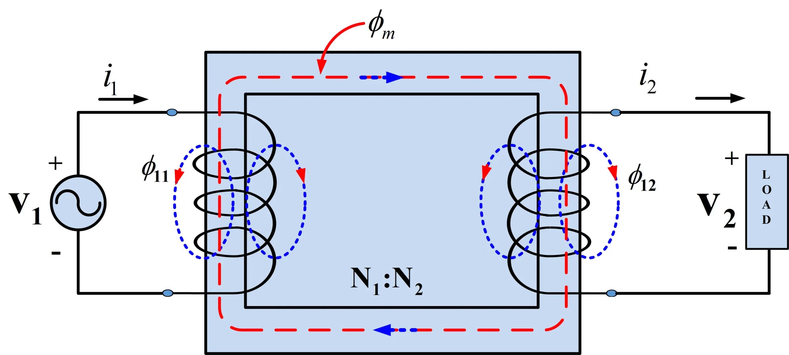
Figure 1: An Actual Transformer
Thus, equation (1) reduces to
\[\begin{matrix} {{\nu }_{1}}={{R}_{1}}{{i}_{1}}+{{N}_{1}}\frac{d{{\phi }_{11}}}{dt}+{{N}_{1}}\frac{d{{\phi }_{m}}}{dt} & {} & (3) \\\end{matrix}\]
Since the leakage flux is a linear function of the primary current i1, the second term on the right-hand side of equation (3) may be expressed in terms of the inductance of the primary winding. Thus,
\[\begin{matrix} {{\nu }_{1}}={{R}_{1}}{{i}_{1}}+{{L}_{1}}\frac{d{{i}_{1}}}{dt}+{{N}_{1}}\frac{d{{\phi }_{m}}}{dt} & {} & (4) \\\end{matrix}\]
The secondary circuit is considered next. From Fig. 1, the voltage equation in the secondary may be written as follows:
\[\begin{matrix} {{\nu }_{2}}=-{{R}_{2}}{{i}_{2}}+{{N}_{2}}\frac{d{{\lambda }_{2}}}{dt}=-{{R}_{2}}{{i}_{2}}+{{N}_{2}}\frac{d{{\phi }_{2}}}{dt} & {} & (5) \\\end{matrix}\]
From the flux direction, the secondary flux may be represented by the difference between the mutual flux and the secondary leakage flux:
\[\begin{matrix} {{\phi }_{2}}={{\phi }_{m}}-{{\phi }_{12}} & {} & (6) \\\end{matrix}\]
Substituting equation (6) into (5) yields
\[\begin{matrix} {{\nu }_{2}}=-{{R}_{2}}{{i}_{2}}-{{N}_{2}}\frac{d{{\phi }_{12}}}{dt}+{{N}_{2}}\frac{d{{\phi }_{m}}}{dt} & {} & (7) \\\end{matrix}\]
Similarly, the leakage flux is a linear function of the secondary current i2. Thus, equation (7) may be written using the inductance of the secondary winding as:
\[\begin{matrix} {{\nu }_{2}}=-{{R}_{2}}{{i}_{2}}-{{L}_{2}}\frac{d{{i}_{2}}}{dt}+{{N}_{2}}\frac{d{{\phi }_{m}}}{dt} & {} & \left( 8 \right) \\\end{matrix}\]
In equations (4) and (8), the last terms represent the induced voltages across the primary and secondary windings, respectively; that is,
\[\begin{matrix} {{e}_{1}}={{N}_{1}}\frac{d{{\phi }_{m}}}{dt} & {} & \left( 9 \right) \\\end{matrix}\]
\[\begin{matrix} {{e}_{2}}={{N}_{2}}\frac{d{{\phi }_{m}}}{dt} & {} & \left( 10 \right) \\\end{matrix}\]
Dividing equation (9) by (10) yields the voltage ratio:
\[\begin{matrix} \frac{{{e}_{1}}}{{{e}_{2}}}=\frac{{{N}_{1}}}{{{N}_{2}}}=a & {} & \left( 11 \right) \\\end{matrix}\]
Figure 2 shows the equivalent circuit of the two-winding transformer of Fig.1. The circuit elements that are used to model the core magnetization and the core losses can be added to either the primary side or the secondary side. In Fig.2, the inductor Lm1 representing the core magnetization and the resistor Rc1 representing the core losses (hysteresis and eddy current losses) have been connected in parallel and located in the primary side of the transformer equivalent circuit.
The core-related circuit elements Rc1 and Lm1 are usually determined at rated voltage and are referred to the primary side in Fig.2. They are assumed to remain essentially constant when the transformer operates at, or near, rated conditions.
- You May Also Read: Transformer Losses and Efficiency Calculation
Transformer Equivalent Circuit in Phasor Form
In phasor form, the transformer equivalent circuit takes the form shown in Fig.3. The reactances are derived by multiplying the inductances by the radian frequency$\omega =2\pi f$, where f is the frequency. The turns ratio a= N1/N2 is approximately equal to the voltage ratio V1/V2, the ratio of the rated primary voltage to the rated secondary voltage provided by the manufacturer.
Figure 2: Equivalent Transformer Circuit
Figure 3: Transformer Equivalent Circuit in Phasor Form
A phasor diagram for a lagging power factor (inductive) load connected across the secondary of the transformer of Fig.3 is shown in Fig.4.
The notation used is as follows:
\[\begin{array}{*{35}{l}} {{\text{E}}_{\text{1}}}=\text{ }primary\text{ }induced\text{ }voltage \\ {{\text{E}}_{\text{2}}}=\text{ }secondary\text{ }induced\text{ }voltage \\ {{\text{V}}_{\text{1}}}=\text{ }primary\text{ }terminal\text{ }voltage~~~~~~~~~~~~~~~~~ \\ {{\text{V}}_{\text{2}}}=\text{ }secondary\text{ }terminal,\text{ }voltage \\ \begin{align} & {{\text{I}}_{\text{1}}}=~primary\text{ }current \\ & {{\text{I}}_{\text{1}}}=~Secondary\text{ }current \\\end{align} \\ {{\text{I}}_{\text{e}}}=\text{ }excitation\text{ }current \\ {{\text{I}}_{\text{m}}},\text{ }{{X}_{m}}=\text{ }magnetizing\text{ }current\text{ }and\text{ }reactance \\ {{\text{I}}_{\text{c}}},\text{ }{{R}_{c}}=\text{ }current\text{ }and\text{ }resistance\text{ }representing\text{ }core\text{ }loss \\ ~~~{{R}_{1}}=\text{ }resistance\text{ }of\text{ }the\text{ }primary\text{ }winding \\ ~~~~{{R}_{2}}=\text{ }resistance\text{ }of\text{ }the\text{ }secondary\text{ }winding \\ ~~~~{{X}_{1}}=\text{ }primary\text{ }leakage\text{ }reactance \\ ~~~~{{X}_{2}}=\text{ }secondary\text{ }leakage\text{ }reactance \\\end{array}\]
Equivalent Circuit of Transformer Referred to Primary Side and Secondary Side
In the transformer equivalent circuit of Fig.3, the ideal transformer can be moved out to the right or to the left of the equivalent circuit by referring all quantities to the primary or secondary, respectively, as shown in Fig.5. This is almost always done because of the great simplicity it introduces in transformer analysis.
Figure 4: Transformer Equivalent Circuit Phasor Diagram
Figure 5 (a): Transformer equivalent circuit referred to Primary Side
Figure 5 (b): Transformer equivalent circuit referred to Secondary Side
Approximate Equivalent Circuit of Transformer Referred to Primary and Secondary Side
The derivation of approximate equivalent circuits begins with the diagrams shown in Fig.5. All quantities have been referred to the same side of the transformer, and the ideal transformer may be omitted from the equivalent circuit.
- The first step in the simplification process is to move the shunt magnetization branch from the middle of the T circuit to either the primary or secondary terminal, as shown in Fig.6 (a) and (b). This step neglects the voltage drop across the primary or secondary winding caused by the exciting current. The voltage drop caused by the load component of the current is still included, of course.

Figure 6: Approximate Equivalent Circuit (a) and (b)
2. The primary and secondary winding resistances are combined to give either the equivalent resistance referred to the primary side ${{R}_{e1}}={{R}_{1}}+{{a}^{2}}{{R}_{2}}$ or the equivalent resistance referred to the secondary side${{R}_{e2}}={}^{{{R}_{1}}}/{}_{{{a}^{2}}}+{{R}_{2}}$.
3. Similarly, the primary and secondary winding reactances are combined to obtain either the equivalent reactance referred to the primary side ${{X}_{e1}}={{X}_{1}}+{{a}^{2}}{{X}_{2}}$ or the equivalent reactance referred to the secondary side${{X}_{e2}}={}^{{{X}_{1}}}/{}_{{{a}^{2}}}+{{X}_{2}}$.
4. The next step in deriving the approximate equivalent circuit is the deletion of the shunt magnetizing branch completely. Thus, the transformer equivalent circuit reduces to a simple equivalent series impedance referred to either primary or secondary, as shown in Fig .6 c and d.

Figure 7: Approximate Equivalent Circuit (c) and (d)
- You May Also Read: Transformer Working Principle | How Transformer Works
Equivalent Circuit of Transformer Referred to Primary and Secondary Side Key Takeaways
Understanding and modeling a non-ideal transformer using an equivalent circuit is essential for accurately analyzing real-world transformer behavior. These models incorporate practical elements such as winding resistances, leakage fluxes, and core losses—factors that significantly impact transformer performance under load. By representing these effects through an equivalent circuit, engineers and designers can predict voltage drops, efficiency losses, and power transfer characteristics more precisely. This becomes especially important in applications like power distribution, electrical equipment design, and industrial automation, where precise voltage regulation and energy efficiency are critical.