The article discusses the performance and power analysis of synchronous generator, focusing on round-rotor and salient-pole machines. It covers key concepts such as phasor diagrams, power equations, power angle stability, and the distinction between magnet and reluctance power contributions.
Most of the electricity we use on a daily basis is created by synchronous generators. Synchronous generators produce constant-frequency power and can operate at both leading and lagging power factors.
Delivered power for the round-rotor machine
From figure 1, we can write a voltage equation:
$\begin{matrix} {{E}_{a}}={{V}_{t}}+jI{{X}_{s}} & {} & \left( 1 \right) \\\end{matrix}$
In Figure 1, the terminal voltage has been chosen as the reference phasor. The angle between the terminal voltage and the generated voltage is the power angle, designated by δ.
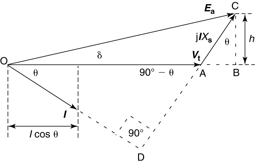
Figure 1: Phasor diagram for the synchronous generator.
The current in Figure 1 has been arbitrarily chosen to be lagging by the angle θ, but all of the results we derive next apply regardless of the power factor.
The second term on the right-hand side of equation 1 contains the factor j, which represents a complex number with a magnitude of 1 and an angle of 90°. Thus, when we multiply the current by jXs, the resulting phasor, jIXs, leads the current by 90°.
As shown in Figure 1, the angle formed at the intersection of the extension of the current phasor with the extension of the phasor jIXs is a right angle. This provides a very convenient way to construct the phasor diagram. Once the terminal voltage and current are drawn, the right triangle OAD is formed and the line DA indicates the direction of the voltage drop across the synchronous reactance.
Triangle OAD is a right triangle, so the angle OAD is (90°-θ). Dropping a line from the tip of the generated voltage (point C) that is perpendicular to the extension of the terminal voltage (line AB) forms a second right triangle, ABC, that is geometrically similar to triangle OAD since two sides of each are formed by intersecting lines. Thus, the angle ACB is θ, the power factor angle.
Side BC of triangle ABC is the height of the generated voltage above the terminal voltage and is designated by h in Figure 1. The distance h can be found not only in terms of the current from triangle ABC but also in terms of the generated voltage since triangle OBC is also a right triangle. In particular,
$\begin{matrix} h={{E}_{a}}\sin \delta =I{{X}_{s}}\cos \theta & {} & \left( 2 \right) \\\end{matrix}$
For the terminal voltage and current shown in Figure 1, we could solve for the power delivered per phase from the machine using the power formula:
$\begin{matrix} {{P}_{1\phi }}={{V}_{t}}I\cos \theta & {} & \left( 3 \right) \\\end{matrix}$
From equation 2, we can solve for Icosθ in terms of the generated voltage and the power angle, δ. Substituting the results into equation 3 yields
$\begin{matrix} {{P}_{1\phi }}=\frac{{{V}_{t}}{{E}_{a}}}{{{X}_{s}}}\sin \delta & {} & \left( 4 \right) \\\end{matrix}$
Since there are three phases, the total three-phase power from the machine is
$\begin{matrix} {{P}_{3\phi }}=3\frac{{{V}_{t}}{{E}_{a}}}{{{X}_{s}}}\sin \delta & {} & \left( 5 \right) \\\end{matrix}$
Equation 5 is an extremely important equation for the synchronous machine because it relates the power delivered to the generated and terminal voltages and the angle between them. This equation shows clearly why the angle δ is called the power angle.
Figure 2 shows a normalized plot of equation 5. The power delivered by the machine varies as the sine of the power angle.
Increasing the power angle increases the amount of power delivered from the machine until the power angle reaches 90°. If the power angle moves past 90°, the machine delivers less power as the angle increases. Attempting to add more load as the power angle increased past 90° would cause the rotor field to lose synchronism with the stator rotating field, resulting in unstable operation, called pole slipping. Pole slipping can be very detrimental to a synchronous machine.

Figure 2: Power delivered by a synchronous generator as a function of the power angle.
Power is related to torque by the rotational speed of the rotor:
$\begin{matrix} P={{\omega }_{s}}T & {} & \left( 6 \right) \\\end{matrix}$
Therefore, the electromagnetic torque of the machine is also a function of the power angle, and the maximum value of torque for the round-rotor machine occurs at a power angle of 90°, assuming the generated and terminal voltages are held fixed.
A derivation similar to equations 2 through 5 results in an expression for the reactive power delivered or absorbed by the machine:
$\begin{matrix} {{Q}_{3\phi }}=3\frac{{{V}_{t}}{{E}_{a}}\cos \delta -V_{t}^{2}}{{{X}_{s}}} & {} & \left( 7 \right) \\\end{matrix}$
Power and torque in the salient- pole synchronous generator
The power and torque calculated by equations 5 and 6 are a result of the interaction of the magnetic fields of the rotor and the stator. This interaction is present in all synchronous machines whether round-rotor or salient-pole and is sometimes called the magnet power.
In a round-rotor machine, all of the power and torque are due to the magnet power; however, in a salient-pole machine, there is another mechanism for creating the torque that must be included.
As discussed earlier, the air gap in a salient-pole machine is not uniform, which means the reluctance of the air gap varies as a function of position on the rotor. Thus, the salient-pole synchronous machine cannot be modeled by a single value of synchronous reactance. Instead, two values are used to model it—the direct-axis reactance, Xd, and the quadrature-axis reactance, Xq.
Magnetic flux prefers a low reluctance path, so even if the field was turned off on the salient-pole rotor, there would be a force that would try to align the direct axis of the rotor with the rotating magnetic field. Thus, we have a reluctance torque in the salient-pole synchronous machine, which by equation 6 creates additional power from the machine.
Note that there are two ways to obtain the low reluctance path with the salient-pole rotor; i.e., the rotor could be moved 180 electrical degrees and still have a low reluctance path. This means the reluctance torque and power vary as a function of twice the power angle. The derivation of the power in a salient-pole synchronous generator is beyond the scope of this topic but results in the following equation:
$\begin{matrix} {{P}_{3\phi }}=3\frac{{{V}_{t}}{{E}_{a}}}{{{X}_{s}}}\sin \delta +V_{t}^{2}\left( \frac{{{X}_{d}}-{{X}_{q}}}{2{{X}_{d}}{{X}_{q}}} \right) & {} & \left( 8 \right) \\\end{matrix}$
The first term on the right-hand side of equation 8 is the magnet power, and the second term is the reluctance power.
Note that for the round-rotor machine the direct- and quadrature-axis reactances are equal, so the reluctance power is zero and equation 8 reduces to equation 5.
Figure 3 shows plots of the magnet power, reluctance power, and total power for a salient-pole rotor. The reluctance power and torque peak at a power angle of 45°, causing a shift of the stability limit for the machine. In this case, the reluctance power is 15% of the magnet power, and the peak power is developed at a power angle of about 11°.
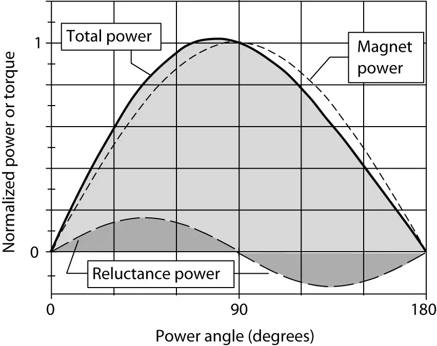
Figure 3: Plot of power vs. power angle for a salient-pole synchronous generator.
Synchronous Generator Key Takeaways
Understanding the performance and power characteristics of synchronous generators—particularly the differences between round-rotor and salient-pole machines—is essential for efficient design and operation in real-world electrical power systems. These machines are the backbone of electricity generation in power plants, providing constant-frequency power required for industrial, commercial, and residential use. The power equations derived, such as those involving the power angle (δ), help engineers predict the delivered power and ensure stable operation. Moreover, distinguishing between magnet power and reluctance power is crucial for optimizing performance in salient-pole machines, which are widely used in hydroelectric applications due to their low-speed operation.