The article explains the concept of exciting current in transformers, detailing its non-sinusoidal nature, harmonic content, and components related to core losses and magnetizing effects, along with an equivalent circuit model. It also discusses inrush current, a high transient current occurring during transformer energization due to core saturation, which is important for protective device sizing.
A practical transformer is not ideal and will require current into the primary winding to establish the flux in the core. The current that establishes the flux is called the exciting current. The exciting current magnitude is usually about 1%-5% of the rated current of the primary.
By Faraday’s law, if we apply a sinusoidal voltage to the transformer, then the flux will also be sinusoidal. However, because of the nonlinearity of the B-H curve for the iron core, the current will not be sinusoidal if the flux is sinusoidal. In addition, the current will be out of phase with the flux due to hysteresis in the iron. Recall that
$\begin{matrix} \phi=B A & and & H=\frac{NI}{\ell } \\\end{matrix}$
Thus, a plot of ɸ vs. I has the same shape as the B-H curve (hysteresis loop). Figure 1 shows a geometrical construction of the exciting current.
The top left curve shows the flux as a function of time (a sine wave). The top right curve shows the flux vs. current hysteresis loop, which represents a map between flux and current. If we know the flux, we can use the map to find out how much current is required.
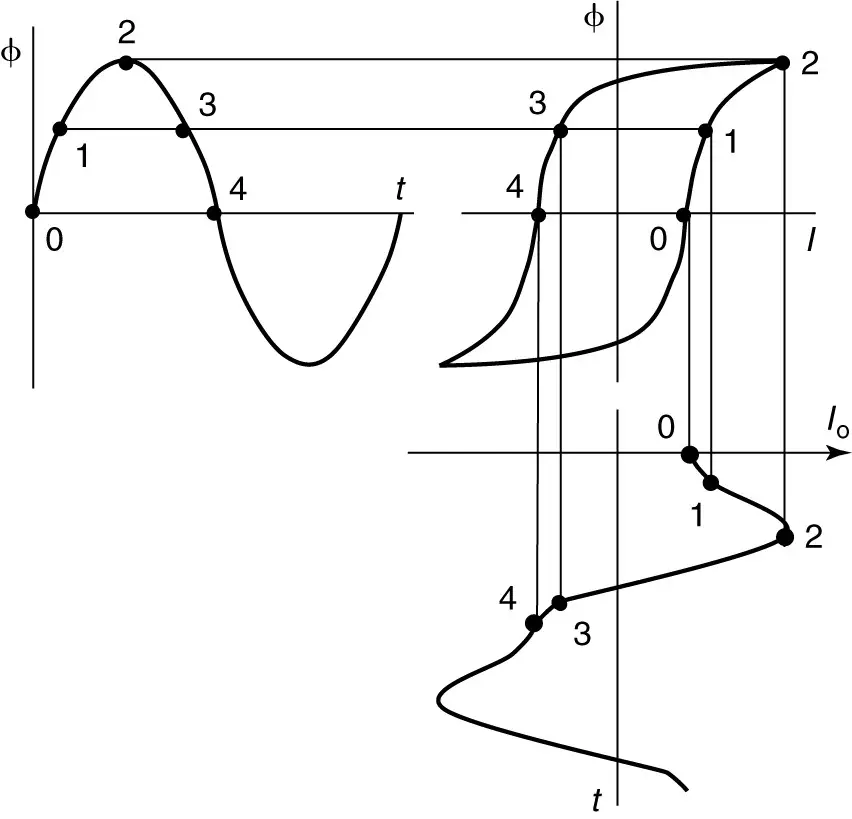
Figure 1 Geometrical construction of transformer exciting current.
Starting at t = 0 (the point indicated by 0), the flux is zero and increasing. Going over to the ɸ vs. I hysteresis loop, we find that when the flux is zero and increasing, some exciting current is required (also indicated by a 0). Thus, the current is out of phase with the flux since they are not both zero at the same time.
Finally, at the bottom right, we can plot the exciting current as a function of time. At t = 0, we plot the current we found, by dropping straight down. Sometime later, the flux is at point 1 and still increasing. Again, we can come across and down and plot the current at the proper time. The process is repeated for the points labeled 2, 3, and 4.
The current is clearly not sinusoidal, but it is periodic. Like any periodic waveform, it could be represented by a Fourier series.
As an example of the harmonic content in the exciting current, Figure 2 shows a fundamental sine wave with an amplitude of 1.0 and a third harmonic cosine with an amplitude of 0.25. Note that when the two are added together, the shape is similar to the exciting current waveform. Thus, as we might expect, there is a significant amount of the third harmonic in the exciting current.
Third harmonics are particularly bad because they are in phase in the three phases of the power system. Thus, they result in circulating currents or neutral currents in a three-phase transformer.

Figure 2 a. The harmonic content of exciting current. b. Measured exciting current.
Although the exciting current is nonsinusoidal, we can define and calculate an rms value for it, as shown by equation 1:
$\begin{matrix} {{I}_{o,rms}}=\sqrt{\frac{\int\limits_{0}^{2\pi }{{{\left[ {{i}_{o}}\left( \omega t \right) \right]}^{2}}d\left( \omega t \right)}}{2\pi }} & {} & \left( 1 \right) \\\end{matrix}$
Fortunately, we do not have to attempt to do this calculation. Instead of using the complete Fourier series for the exciting current, we will approximate it by a single component at the fundamental (60 Hz) frequency.
We could measure the no-load current into a transformer with a true rms ammeter to determine this value, and then represent that single component by a phasor diagram, as shown in Figure 3.
We saw from the geometric construction that the exciting current was not in phase with the flux. The voltage is 90° ahead of the flux, since the voltage is the derivative of the flux, and the exciting current is between them.
Since the exciting current phasor lies between the voltage phasor and the flux phasor, we can separate the current into two components, one in phase with the voltage and one in phase with the flux.
The component of current in phase with the voltage, lfe, represents real power being consumed and is called the core-loss current.
The component of current in phase with the flux, lm, represents reactive power and is called the magnetizing current.
Given these two components of current, we can draw an equivalent circuit consisting of a resistance and inductive reactance in parallel, as shown in Figure 4.
The resistance, Rfe, consumes real power corresponding to the core losses of the transformer. The designation Rc is also frequently used for this element. The inductive reactance, Xm, draws the current used to create the magnetic field in the transformer core.
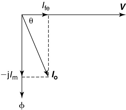
Figure 3 Phasor diagram of exciting current.
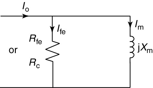
Figure 4 Equivalent circuit of transformer core.
We can calculate values for Rfe and Xm. With no load on the transformer, measure the rms current into the transformer, the input voltage, and the real power into the transformer. The product of the voltage and current gives the apparent power, S. Since the real power is known, we can find the power factor and the impedance angle. The elements can then be calculated.
Exciting power
Note that the apparent power to excite the core is given by the product of the rms voltage and the rms exciting current.
Typically, the exciting current is a few percents of full-load current. But ${{A}_{c}}{{\ell }_{c}}$(A=core area, l= core length) is the volume of the core, so the apparent exciting power is proportional to the size of the core. Similarly, we can find the real exciting power using the core loss component of the exciting current. It is also proportionate to the size of the core. Manufacturers of electrical steel provide curves of exciting power and core loss as a function of magnetic flux density and frequency.
Inrush Current in Transformer
In the geometric construction of the magnetizing current, we assumed the voltage applied to the primary coil was a cosine wave. Since the flux is proportionate to the integral of the voltage, ɸ had the form of a sine wave.
Suppose, instead, the voltage applied to the primary was a sine wave; i.e., the voltage was applied to the coil when it crosses through zero, as shown in Figure 5. Also, assume for now that there is no residual magnetism in the core.
The flux, being the integral of voltage, should be a negative cosine wave, as shown by the curve labeled ɸss (steady-state flux). Thus, the flux should be at a negative peak as shown in Figure 1. However, the flux was zero at time zero; therefore, it cannot be anything other than zero immediately after the voltage is applied because an instantaneous change of flux would require an impulse voltage. So the flux begins at zero and rises with the form of a negative cosine, as shown by the curve labeled ɸtransient.
At $\omega t=\pi /2$, the flux has increased to its normal peak value, but the voltage is still positive, so the flux must continue to increase, eventually reaching twice its peak value at $\omega t=\pi $.
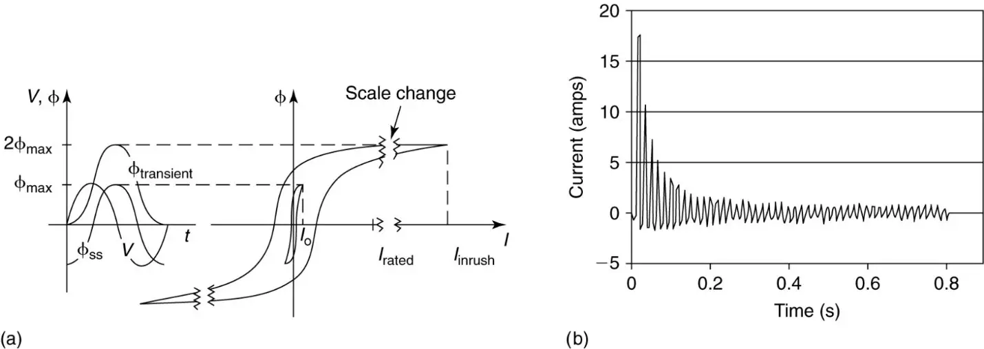
Figure 5 a. Illustration of inrush current. b. Measured inrush current.
Attempting to achieve this high level of flux will drive the device far into saturation because most electromagnetic devices are designed to normally operate near the knee of the B-H curve.
The right- hand curve of Figure 1 illustrates what occurs. At normal peak values of ɸ, the magnetizing current has a peak value that is a small percentage of rated current. But driving the transformer far into saturation can result in currents as high as 12 times rated current. This phenomenon is called the inrush current and must be taken into consideration when sizing fuses or circuit breakers on the primary of the transformer.
Exciting Current in Transformer Key Takeaways
understanding the exciting current and inrush current in transformers is essential for their effective application and reliable operation. The non-sinusoidal nature and harmonic content of the exciting current impact transformer losses, efficiency, and power quality, while the equivalent circuit model helps in accurately predicting transformer behavior under no-load conditions. Inrush current, being a large transient surge during energization caused by core saturation, is critical for the correct selection and coordination of protective devices such as fuses and circuit breakers to prevent nuisance tripping or damage. These concepts ensure transformers are designed, operated, and protected properly, enabling stable power delivery in electrical systems across industrial, commercial, and residential applications.