The article explains the swing equation, a key mathematical formula that models the dynamic behavior of synchronous generators in power systems. It outlines the derivation process, starting from Newton’s law of rotation and incorporating angular position and velocity. The swing equation describes how rotor angle acceleration is influenced by active power imbalances, helping to assess the stability of power systems during transient disturbances.
What is a Swing Equation?
The motion of a synchronous machine is governed by Newton’s law of rotation, which states that the product of the moment of inertia times the angular acceleration is equal to the net accelerating torque. Mathematically, this may be expressed as follows:
$\begin{matrix} J\alpha ={{T}_{a}}={{T}_{m}}-{{T}_{e}} & {} & \left( 1 \right) \\\end{matrix}$
Equation 1 may also be written in terms of the angular position as follows:
$\begin{matrix} J\frac{{{d}^{2}}{{\theta }_{m}}}{d{{t}^{2}}}={{T}_{a}}={{T}_{m}}-{{T}_{e}} & {} & \left( 2 \right) \\\end{matrix}$
where
J = moment of inertia of the rotor
Ta = net accelerating torque or algebraic sum of all torques acting on the machine
Tm = shaft torque corrected for the rotational losses including friction and windage and core losses
Te = electromagnetic torque
Note: By convention, the values of Tm and Te are taken as positive for generator action and negative for motor action.
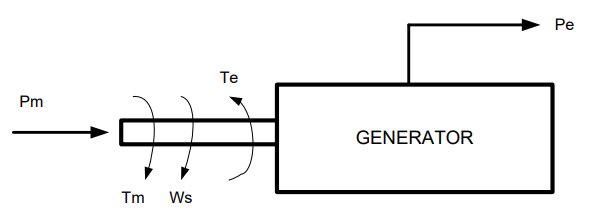
Figure 1. Power Flow in a Synchronous Generator
Swing Equation Derivation
For stability studies, it is necessary to find an expression for the angular position of the machine rotor as a function of time t. However, because the displacement angle and relative speed are of greater interest, it is more convenient to measure angular position and angular velocity with respect to a synchronously rotating reference frame with a synchronous speed of${{\omega }_{sm}}$. Thus, the rotor position may be described by the following:
$\begin{matrix} {{\theta }_{m}}={{\omega }_{sm}}+{{\delta }_{m}} & {} & \left( 3 \right) \\\end{matrix}$
The derivatives of θm may be expressed as
$\begin{align} & \begin{matrix} \frac{d{{\theta }_{m}}}{dt}={{\omega }_{sm}}+\frac{d{{\delta }_{m}}}{dt} & {} & \left( 4 \right) \\\end{matrix} \\ & \begin{matrix} \frac{{{d}^{2}}{{\theta }_{m}}}{d{{t}^{2}}}=\frac{{{d}^{2}}{{\delta }_{m}}}{d{{t}^{2}}} & {} & \left( 5 \right) \\\end{matrix} \\\end{align}$
Substituting Equation 5 into Equation 2 yields
$J\begin{matrix} \frac{{{d}^{2}}{{\delta }_{m}}}{d{{t}^{2}}}={{T}_{a}}={{T}_{m}}-{{T}_{e}} & {} & \left( 6 \right) \\\end{matrix}$
Multiplying Equation 6 by the angular velocity of the rotor transforms the torque equation into a power equation. Thus,
$J{{\omega }_{m}}\begin{matrix} \frac{{{d}^{2}}{{\delta }_{m}}}{d{{t}^{2}}}={{\omega }_{m}}{{T}_{a}}={{\omega }_{m}}{{T}_{m}}-{{\omega }_{m}}{{T}_{e}} & {} & \left( 7 \right) \\\end{matrix}$
Replacing ${{\omega }_{m}}T$ by P and $J{{\omega }_{m}}$ by M, the so-called swing equation is obtained. The swing equation describes how the machine rotor moves, or swings, with respect to the synchronously rotating reference frame in the presence of a disturbance, that is, when the net accelerating power is not zero.
$M\begin{matrix} \frac{{{d}^{2}}{{\delta }_{m}}}{d{{t}^{2}}}={{P}_{a}}={{P}_{m}}-{{P}_{e}} & {} & \left( 8 \right) \\\end{matrix}$
where
M = Jω = inertia constant
Pa = Pm– Pe = net accelerating power
Pm = ωTm = shaft power input corrected for the rotational losses
Pe = ωTe = electrical power output corrected for the electrical losses
It may be noted that the inertia constant was taken equal to the product of the moment of inertia J and the angular velocity ωm, which actually varies during a disturbance. Provided the machine does not lose synchronism, however, the variation in ωm is quite small. Thus, M is usually treated as a constant.
Another constant, which is often used because its range of values for particular types of rotating machines is quite narrow, is the so-called normalized inertia constant H. It is related to M as follows:
$\begin{matrix} H=\frac{1}{2}\frac{M{{\omega }_{sm}}}{{{S}_{rated}}}{}^{MJ}/{}_{MVA} & {} & \left( 9 \right) \\\end{matrix}$
Solving for M from Equation 9 and substituting into 8 yields the swing equation expressed in per unit. Thus,
\[\frac{2H}{{{\omega }_{sm}}}\begin{matrix} \frac{{{d}^{2}}{{\delta }_{m}}}{d{{t}^{2}}}=\frac{{{P}_{a}}}{{{S}_{rated}}}=\frac{{{P}_{m}}}{{{S}_{rated}}}-\frac{{{P}_{e}}}{{{S}_{rated}}} & {} & \left( 10 \right) \\\end{matrix}\]
It may be noted that the angle δm and angular velocity ωm in Equation 10 are expressed in mechanical radians and mechanical radians per second, respectively. For a synchronous generator with p poles, the electrical power angle and radian frequency are related to the corresponding mechanical variables as follows:
$\begin{matrix} \begin{align} & \delta \left( t \right)=\frac{p}{2}{{\delta }_{m}}\left( t \right) \\ & \omega \left( t \right)=\frac{p}{2}{{\omega }_{m}}\left( t \right) \\\end{align} & {} & \left( 11 \right) \\\end{matrix}$
Similarly, the synchronous electrical radian frequency is related to synchronous angular velocity as follows:
$\begin{matrix} {{\omega }_{s}}=\frac{p}{2}{{\omega }_{sm}} & {} & \left( 12 \right) \\\end{matrix}$
Therefore, the per-unit swing equation of Equation 10 may be expressed in electrical units and takes the form of Equation 13.
$\frac{2H}{{{\omega }_{s}}}\begin{matrix} \frac{{{d}^{2}}\delta }{d{{t}^{2}}}={{P}_{a}}={{P}_{m}}-{{P}_{e}} & {} & \left( 13 \right) \\\end{matrix}$
Depending on the unit of the angle δ, Equation 13 takes the form of either Equation 14 or 15. Thus, the per-unit swing equation takes the form:
$\frac{H}{\pi f}\begin{matrix} \frac{{{d}^{2}}\delta }{d{{t}^{2}}}={{P}_{a}}={{P}_{m}}-{{P}_{e}} & {} & \left( 14 \right) \\\end{matrix}$
When δ is in electrical degrees, or
$\frac{H}{180f}\begin{matrix} \frac{{{d}^{2}}\delta }{d{{t}^{2}}}={{P}_{a}}={{P}_{m}}-{{P}_{e}} & {} & \left( 15 \right) \\\end{matrix}$
When δ is in electrical degrees.
When a disturbance occurs, an unbalance in the power input and power output ensues, producing a net accelerating torque. The solution of the swing equation in the form of the differential equation of (14) or (15) is appropriately called the swing curve δ (t).
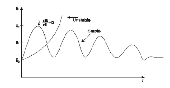
Figure 2. Swing Curve: A plot of δ (t)
Swing Equation Importance
The swing equation is of significant importance in the analysis and stability assessment of power systems. It is a mathematical equation that describes the dynamic behavior of synchronous generators in power systems during transient conditions.
The swing equation helps determine the rotor angle stability and the response of synchronous generators to disturbances such as faults or sudden changes in load. By modeling the mechanical and electrical dynamics of the generator, the swing equation provides insights into the system’s transient stability and the ability to maintain synchronism.
The importance of the swing equation lies in its ability to assess the stability of power systems and guide control actions to maintain stable operation. By analyzing the swing equation, engineers can evaluate the critical clearing time, which is the time needed for the system to recover from a disturbance and regain stability.
Understanding the swing equation allows power system operators and engineers to design appropriate control strategies and protective schemes to prevent cascading failures, blackouts, or voltage collapse. It helps in optimizing system performance, determining appropriate control settings, and ensuring the reliable and secure operation of power systems.
Overall, the swing equation plays a crucial role in maintaining the stability and resilience of power systems, contributing to the efficient and reliable generation, transmission, and distribution of electrical energy.
Swing Equation FAQs
What is the swing equation?
The swing equation is a mathematical equation that describes the dynamic behavior of synchronous generators in power systems during transient conditions. It relates the acceleration of the generator rotor angle to the active power imbalance in the system.
Why is the swing equation important?
The swing equation is important because it helps assess the stability of power systems during transient events. It allows engineers to analyze the system’s response to disturbances, determine critical clearing time, and design control strategies to maintain stable operation.
What does the swing equation tell us about power system stability?
The swing equation provides insights into the stability of power systems by determining the rotor angle stability and the system’s ability to maintain synchronism. It helps identify potential stability issues and guides control actions to prevent cascading failures or voltage collapse.
How is the swing equation used in power system analysis?
The swing equation is used in power system analysis to simulate the dynamic behavior of synchronous generators and assess system stability. It is incorporated into transient stability studies and helps engineers make informed decisions about system design, control strategies, and protective schemes.
What parameters are involved in the swing equation?
The swing equation involves parameters such as the moment of inertia of the generator rotor, the electrical power output, system frequency, and damping coefficients. These parameters determine the response of the generator to disturbances and play a crucial role in stability analysis.
Can the swing equation be used to predict the stability of power systems?
Yes, the swing equation, along with appropriate system modeling and simulation techniques, can help predict the stability of power systems. By analyzing the swing equation, engineers can identify potential stability issues and take preventive measures to ensure reliable and secure operation.