This article examines transient stability in large interconnected power systems and their four operating states.
Power system stability refers to the ability of the various synchronous machines in the system to remain in synchronism or stay in step, with each other following a disturbance. Stability may be classified as steady-state, dynamic, or transient stability.
Steady-state stability refers to the ability of the various machines to regain and maintain synchronism after a small and slow disturbance, such as a gradual change in load.
Transient stability in a power system is stability after a sudden large disturbance such as a fault, loss of a generator, a switching operation, and a sudden load change.
Dynamic stability is the case between steady-state and transient stability, and the period of study is much longer so that the effects of regulators and governors may be included.
Consider the two-machine power system shown in Figure 1. Each machine may be represented as a constant emf in series with a synchronous reactance and negligible resistance. Assume that the machine on the left acts as a generator and the other machine acts as a motor. The emf’s may be expressed in polar form as follows:
$\begin{matrix} \begin{align} & {{E}_{g}}=\left| {{E}_{^{g}}} \right|\angle \delta \\ & {{E}_{m}}=\left| {{E}_{^{m}}} \right|\angle {{0}^{o}} \\\end{align} & {} & \left( 1 \right) \\\end{matrix}$
The current flowing in the circuit is given by
$\begin{matrix} I=\frac{{{E}_{g}}-{{E}_{m}}}{j{{X}_{T}}}=\frac{\left| {{E}_{g}} \right|\angle \delta -\left| {{E}_{m}} \right|\angle {{0}^{o}}}{j{{X}_{T}}} & {} & \left( 2 \right) \\\end{matrix}$
Where
\[{{X}_{T}}={{X}_{g}}+{{X}_{e}}+{{X}_{m}}\]
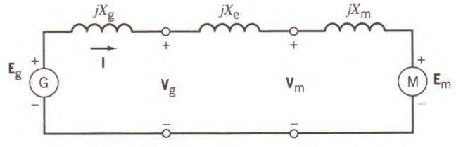
Figure 1. A two-machine power system
The real power delivered by the generator to the motor is found as follows:
\[\begin{matrix} \begin{align} & P=\operatorname{Re}\left[ {{E}_{g}}I* \right] \\ & =\operatorname{Re}\left[ \left( Eg\angle \delta \right){{\left( \frac{\left| {{E}_{g}} \right|\angle \delta -\left| {{E}_{m}} \right|\angle {{0}^{o}}}{j{{X}_{T}}} \right)}^{*}} \right] \\ & =\operatorname{Re}\left[ \frac{E_{g}^{2}}{{{X}_{T}}}\angle {{90}^{o}}-\frac{{{E}_{g}}{{E}_{m}}}{{{X}_{T}}}\angle \delta +{{90}^{o}} \right] \\ & =\frac{{{E}_{g}}{{E}_{m}}}{{{X}_{T}}}Sin\left( \delta \right) \\\end{align} & {} & \left( 3 \right) \\\end{matrix}\]
Thus, it is seen that the power supplied by the generator to the motor varies with the sine of the phase angle difference of the two emf’s, which is also the displacement angle between the two rotors.
The maximum power Pmax that can be transmitted at a steady state from the generator to the motor with the total reactance XT is found from Equation 3 for the case δ = 90°. That is,
$\begin{matrix} {{P}_{\max }}=\frac{{{E}_{g}}{{E}_{m}}}{{{X}_{T}}} & {} & \left( 4 \right) \\\end{matrix}$
Pmax is called the steady-state stability limit. Its value can be raised only by increasing either of the two internal voltages by adjusting their respective excitations or by decreasing the series reactance of the transmission line connecting the two machines.
The plot of the transmitted power versus the displacement angle is called the power-angle curve, and it is illustrated in Figure 2.
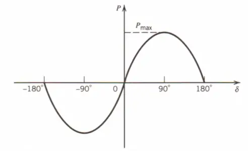
Figure 2. Power-Angle curve
The graph indicates that the system is stable over the operating region -90° < δ < 90°, where the derivative of P with respect to δ is positive, that is,${}^{dP}/{}_{d\delta }>0$; this condition implies that an increase in displacement angle results in an increase in transmitted power.
Consider the two-machine system operating at a steady state at point A on the power-angle curve of Figure 3. Assume that the generator is delivering electrical power Po at an angle δo to the motor, which is driving a mechanical load connected to its shaft.
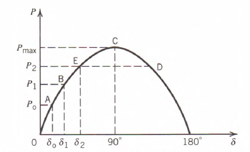
Figure 3. Two machine system operating states.
Case 1.
Suppose that a small increment of shaft load is added to the motor. This net torque tends to retard the motor and its speed decreases, causing an increase in δ. The input power increases correspondingly until equilibrium is obtained at a new operating point B, higher than A.
Case 2.
Suppose that the motor load is increased gradually until point C of maximum power is reached. If the additional load is applied to the motor, δ increases as before and goes beyond 90°. This time, however, instead of an increase in the input power, the input power decreases, which further increases the net retarding torque. This torque retards the motor even faster until it pulls out of step.
Case 3.
Suppose a large increment of load is suddenly applied to the motor. The deficiency in the input will be supplied temporarily by the decrease in kinetic energy. The motor will slow down, increasing δ and the power input. Assuming that the new load is less than Pmax, δ will increase to a new value such that the motor input equals the motor load. When this is reached, the motor is still running slow, thus increasing δ beyond its proper value and producing an accelerating torque that increases the motor speed. However, when the motor regains normal speed, δ may have gone beyond point D so that the motor input is less than the load. This leads to motor pull-out.
Case 4.
Assume for this case that the sudden incremental load is not too great. The motor will regain its normal speed before it becomes too large. The motor speed will continue to increase because of the net accelerating torque and will become greater than normal. When this happens, δ will decrease and again approach its proper value. These oscillations will later die out because of damping torques, and the motor will come to a stable operating condition at point E.
The upper limit to the sudden increment in the load that the rotor can carry without pulling out of step is called the transient stability limit. This is always lower than the steady-state limit and can have different values depending on the nature and magnitude of the disturbance.
Transient Stability in Power System Key Takeaways
Understanding the four operating states of transient stability—along with steady-state and dynamic stability—is crucial for ensuring the reliable operation of large interconnected power systems. These concepts are not just theoretical; they have vital real-world applications in power generation, transmission, and distribution systems. For example, accurate stability assessment helps engineers design systems that can withstand sudden disturbances like faults or load changes without causing cascading failures. It also enables the integration of control mechanisms such as automatic voltage regulators and governors, which play key roles in maintaining synchronism among machines. By analyzing power-angle relationships and rotor dynamics, system operators can predict and mitigate instability, enhancing both operational efficiency and safety.